For the production of ‘Stand By’, I chose to record and edit everything in Cubase 12, as it’s my main DAW and I’m highly familiar with its workflow, shortcuts, and overall layout. The entire project contains nearly 150 tracks, all recorded & edited in Cubase.
When it came to mixing in 3D audio, I decided to begin my spatial audio journey using Ambisonics and Reaper rather than Dolby Atmos. This decision was largely influenced by the IEM Plugin Suite, which offers powerful and intuitive tools for Ambisonics mixing — making the entry into 3D audio more approachable and flexible.
I chose to work with fifth-order Ambisonics for this project to achieve a more accurate and immersive rendering of diffuseness, spaciousness, and spatial depth. While first-order Ambisonics might seem sufficient due to the even nature of diffuse sound fields, in practice, their low spatial resolution leads to high directional correlation during playback, which significantly impairs the perception of these spatial qualities. Higher-order Ambisonics, in contrast, improves the mapping of uncorrelated signals and preserves spatial impressions much more effectively. Psychoacoustic research has shown that an Ambisonic order of three or higher is required to perceptually preserve decorrelation between neighboring loudspeakers, which is crucial for rendering depth and diffuseness. Fifth-order Ambisonics further enhances this, particularly outside the sweet spot, providing a more consistent spatial experience across a larger listening area. As demonstrated in the IEM CUBE, a fifth-order system allows nearly the entire horizontal listening plane—in this case, a 12 × 10 m concert space—to become a valid and perceptually plausible playback zone. [1]
Thus, fifth-order Ambisonics is not only a practical choice for immersive production in larger spaces, but it also strikes an effective balance between spatial resolution, technological complexity, and perceptual benefit [2].
I also had the opportunity to experience this myself during a small listening test we conducted with Matthias Frank. We listened to first-, third-, and fifth-order Ambisonics in a blind comparison and were asked to rate certain spatial parameters like spatial depth or localization. The first order was quite easy to identify due to its limited spatial resolution. However, distinguishing between third- and fifth-order Ambisonics proved to be much more challenging, as the differences were often subtle and less immediately perceptible.
After that, I started with setting up the routing, which was one of the most underestimated parts of this project. Similar to a traditional stereo production, I created a structure of groups and subgroups, but adapted it for Ambisonics. For example, in the drum section, encoding happens at the main drum group via the IEM MultiEncoder. All individual channels are routed into that group, allowing me to process them using conventional stereo plugins before spatializing them — saving both CPU resources and maintaining flexibility in the early mixing stages.
Within the drum routing, I created subgroups for kick, snare, overheads and the droom, allowing for finer control and processing. When dealing with coherent signals, such as double-tracked guitars, I first routed both signals (panned hard L & hard R) into a stereo group to conserve CPU power by processing them together. This group is then routed into a master guitar group that handles Ambisonics encoding. Since the L and R signals remain separated, you can still treat them independently from each other in the encoder. So I can still place them individually in the 3D field — even though they were previously grouped.
I followed the same approach with vocals, organizing them into groups before routing them into the Multiencoder. For specific adlibs, I used the GranularEncoder to create glitchy, scattered spatial effects.
To add a sense of depth and immersion to the vocals, I used a little bit of the FDN Reverb for diffuse reverb and the Room Encoder for some early reflections – all plugins are from the IEM Suite.
Finding this optimal signal flow took quite a bit of time and experimentation. It was a major learning process to understand how to best structure a large session for Ambisonics, and I’m still refining my approach. I’ve already begun mixing in the production studio at IEM, and although there’s certainly still room for improvement, I’m genuinely happy with the current state of the mix. This being my first attempt of a spatial audio mix, I see it as a solid starting point — and I’m excited to continue learning and evolving through hands-on experience.
[1] Franz Zotter und Matthias Frank, Ambisonics: A Practical 3D Audio Theory for Recording, Studio Production, Sound Reinforcement, and Virtual Reality, Bd. 19, Springer Topics in Signal Processing (Cham: Springer International Publishing, 2019), 18–20, https://doi.org/10.1007/978-3-030-17207-7.
In “Stand By”, sound design plays a critical role in reinforcing the song’s emotional core — the psychological entrapment of a toxic relationship, which parallels the patterns of addiction.
To support the emotional arc of Stand By, spatial elements were deliberately positioned behind and around the listener to enhance feelings of tension, disorientation, and emotional overload (more about that below). This approach aligns with findings by Stefanowska and Zieliński (2024), who highlight that rear-positioned and difficult-to-localize sound sources can intensify emotional responses—particularly those associated with discomfort, fear, or psychological distress.[1]
By embracing these psychoacoustic principles, the sound design doesn’t merely illustrate the lyrical content, but actively immerses the listener in the protagonist’s emotional state.
But the key principle that guided my general approach to spatial mixing came from Lasse Nipkow, who emphasized the importance of listener expectation in immersive audio. As he puts it: „Die Leute sind es gewöhnt, dass die Musik vorne spielt, also lasst sie da auch spielen, und packt Wichtiges wie Schlagzeug und Stimme in die vorderen Lautsprecher.[2]“ Translated: “People are used to music playing from the front—so let it play there, and place important elements like drums and vocals in the front loudspeakers.” This mindset shaped my core mixing philosophy. Instead of treating 3D audio as an opportunity to scatter key musical components arbitrarily throughout the sound field, I chose to respect the listener’s intuitive focus. Drums, lead vocals, and harmonic anchors were mostly placed in the front hemisphere to preserve clarity and narrative drive, while the rest of the spatial field—especially the sides, rear, and height—became a playground for emotional and textural enhancement. This balance allowed me to stay immersive without losing musical coherence.
The track begins intentionally narrow and intimate, with the vocal placed front and center and only minimal ad-libs distributed in the surrounding space – Like fleeting thoughts echoing in the periphery. The guitar is slightly off the center, a second guitar plays the octaves of the riff, positioned at low volume on the other side of the room. Subtle rim hits on the rack tom foreshadow the emotional unravelling to come, creeping in like the early signs of danger.
As the second verse enters, the space opens drastically. The full drum kit kicks in with a deep floor tom and a palm-muted guitar part, tracked four times, creates a dense rhythmic bed. Meanwhile, a haunting “Uhh” choir swirls around the listener. This ghostly texture mirrors the psychological fog of emotional abuse — disembodied voices, indifferent and cold, being around you. It captures the emotional numbness and disorientation of dependency: the sense of being surrounded, yet entirely alone.
In the chorus, additional guitar layers are spread wide across the field, amplifying the pressure. Key lyrical lines are doubled with backing vocals:
I’m running in circles ‘Forced to stay’ I want to leave this place ‘But I can’t get away’ It’s frustrating ‘And suffocating’ Promised paradise is a lie — so ‘I’ stay on stand by
After each chorus, the song narrows again, mimicking the push-and-pull dynamic of emotional manipulation — the moments of clarity crushed by renewed confusion. At the line “You made me crazy when you…”, only the lead vocal and one side of the choir remains — before the wall of sound returns suddenly in verse two. This verse escalates with ‘open’ guitar chords (as opposed to the palm-muted ones before), and the drummer expands the groove with the addition of the rack tom.
To emphasize the transition into the second chorus, guitar death notes are layered with the snare hits in the fill — eight tracks in total, radiating outward. The final vocal line “Bursting away” is spatially fractured and scattered in all directions, as if the voice itself is breaking apart under the weight of emotional overload.
Then, after the second chorus, comes the confrontation: four cycles of build-up, followed by four of breakdown. During the build-up, a series of toxic phrases like “After everything I’ve done for you”, “Don’t push me”, “You’re nothing without me” — are placed chaotically into the space. Each one is distorted and spatially placed. Some are passed through granular synthesis (via the IEM Granular Encoder), transforming them into chaotic, stuttering fragments that glitch and scatter unpredictably. It places the listener inside the chaos of an abusive dynamic, where reason disintegrates and confusion dominates.
The tension is increased through a gradual high-cut filter on the guitars — which opens more and more, the closer the breakdown comes. A burning fuse — a literal sound effect — moves around the listener, traveling over their head just before the drop, suggesting both tension and inevitability.
At the start of the breakdown, a sub-drop slams in, marking the collapse. The four breakdown cycles remain true to traditional rock instrumentation but are widened into immersive 3D space.
Then, the moment of illusion arrives. We transition into the stairwell reverb section — a metaphor for the seductive promise of escape. Instead of distributing the stairwell recording (captured with five microphones) across the room, I placed the microphones behind the listener, emphasizing the contrast with the confined front-space. The mix collapses forward again, symbolized by sliding guitars that pan from back to front and the return of the fuse sound, automated to rush toward the listener. It’s the false hope of recovery — crushed by relapse.
The final chorus hits harder. The bass becomes more expressive, adding fills to push the groove forward. The word “suffocation” is no longer static — it’s sung alternately on the left and right, while the lead vocal itself begins to drift toward the backing voices, suggesting emotional fragmentation.
The line “Promised paradise is a lie” is repeated three times in the final chorus. And after that the final lyric line of the song comes – “And I stand on stand by”. A solitary voice. Nothing more. Just like addiction, the emotional trap is isolating. You’re still there. Still connected. But unable to move.
[1] Antonina Stefanowska und Sławomir K. Zieliński, „Spatial sound and emotions: A literature survey on the relationship between spatially rendered audio and listeners’ affective responses“, International Journal of Electronics and Telecommunications, 25. Juni 2024, 297, https://doi.org/10.24425/ijet.2024.149544.
For the bass, we used a Fender Jazz Bass, recorded directly through my Line 6 Helix modeller. We chose a amp simulation that included impulse responses (IRs) replicating the mic’d sound of a cabinet captured with an Audix D6 (typically a kick drum mic) and a Shure SM57. This unusual combination provided exactly what I was looking for: deep, punchy lows from the D6 and more defined highs from the SM57 — a perfect balance for our mix.
With the electric guitars, we kept the 3D audio production in mind throughout the entire process. That’s why we recorded multiple layers to allow for spatial variation during mixing. I played the guitar parts using both a Gibson Les Paul Standard and a custom-built Telecaster — again routed through the Line 6 Helix, which offered us a broad palette of amp and cab simulations with consistent quality.
Vocal Recordings
Vocals were recorded using my Neumann TLM102. We tested several microphones, including the AKG C414 as well as the new version of this microphone, the Austrian Audio OC818. In the end, the TLM102 simply fit Lukas’s voice the best. For certain shouts and accents, we recorded more takes to give us more layering options in the mix.
Backing vocals and harmonies were performed by Clemens (our bassist), Lukas (our lead vocalist), and myself. We used a variety of techniques — including thirds above and below the lead vocal — and occasionally doubled the lead in octaves to add emotional weight or build intensity in specific sections.
We’ve already written eight songs for the album. Every time we move toward recording a new track, we sit down as a band and evaluate which song we want to take out of the pre-production phase and develop further. The last one we recorded was a song called ‘Stand By’. Since we had only recently written it, the energy and momentum around the track were still fresh — we were all highly motivated to fully produce it and spend more time engaging with its emotional and sonic layers. Not all of the songs we’ve written will make it onto the final album, and the writing process is still ongoing. We’re planning to write additional songs over the summer, including sessions with external professional songwriters to expand our creative input and further explore the theme from new perspectives.
Concept of the song
‘Stand By’ is a raw and emotional track that dives deep into the suffocating reality of being trapped in a toxic relationship—a dynamic that mirrors the psychological and emotional patterns often found in addiction. The song paints a vivid picture of circular thinking and emotional dependency: the feeling of giving everything and receiving harm in return, the confusion of being hurt by someone who once promised love, and the inner battle of wanting to leave but being psychologically unable to do so.
The metaphor of being ‘on stand by’ captures a state of paralysis—still connected, still present, but unable to act or move forward. In the context of our concept album on addiction and dependency, this song stands as a powerful metaphor for emotional entrapment. Just like with substance or behavioural addictions, the individual becomes stuck in a loop: knowing something is damaging but feeling incapable of breaking away.
First drafts of the lyrics
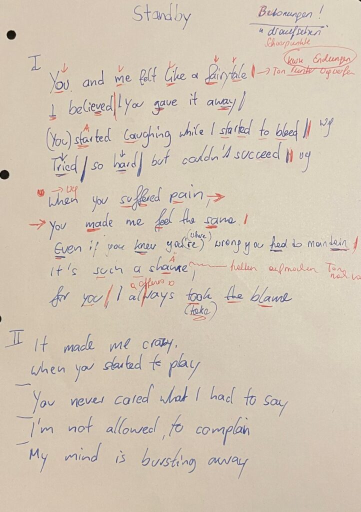
These are the final lyrics of the song ‘Stand by’ – FLAVOR AMP:
[Verse 1] You and me felt like a fairytale, I believed, you gave it away (You) started laughing while I started to bleed Tried so hard fulfilling your needs
[Verse 2] When you suffered pain you made me feel the same Even if you know you’re wrong you had to maintain It’s such a shame For you, I always take the blame
[Chorus 1] I’m running in circles Forced to stay I want to leave this place But I can’t get away It’s frustrating And suffocating Promised paradise is a lie So I stay on stand by
[Verse 3]
It made me crazy when you started to play You never cared what I had to say I’m not allowed to complain My mind is bursting away
[Chorus 2]
I’m running in circles Forced to stay I want to leave this place But I can’t get away It’s frustrating And suffocating Promised paradise is a lie So I stay on stand by
[Build up]
[Breakdown]
[Chorus 3]
I’m running in circles Forced to stay I want to leave this place And I can’t get away It’s frustrating But suffocating [Post Chorus]
Promised paradise is a lie
Promised paradise is a lie So I stay on stand by
With the core structure of the song now in place, we moved on to recording the drums — a key step in shaping the track’s sonic identity.
Our original objective was simple on paper: write a Python utility that would stream real-time heart-rate-variability (HRV) data from a live ECG feed and let a digital-audio workstation turn those numbers into music. The script was expected to read 0.1-second ECG chunks, detect new R-peaks, derive the seven canonical HRV metrics (HR, SDNN, RMSSD, VLF, LF, HF, LF/HF) and hand fresh values to the sound engine every tick. In theory that would allow a performer’s physiology to shape the soundtrack moment-by-moment.
Phase 1 – “print-only” prototype The first proof-of-concept program did nothing but compute the metrics and dump them to the terminal. Because the offline reference library (hrv_plot.py) already produced correct numbers, the live version mimicked its algorithm line-for-line, apart from using a sliding buffer instead of reading the whole file at once. The console printed something every 0.1 s, CPU usage looked negligible, and we assumed we were done.
Phase 2 – OSC transport and the DAW deterrent To let a synthesiser listen, we wrapped the same loop with an Open Sound Control sender. The data reached Ableton Live but required an external bridge, custom track routing and an additional plug-in to map OSC to parameters. Latency was fine, usability was not: every DAW session began with ten minutes of cabling virtual ports. We dropped OSC and decided to embed the information in ordinary MIDI where any host can record or map it instantly.
Phase 3 – first real-time MIDI attempt, and the “melting clock” The next script converted each 0.1-s update into a drum hit on one of sixteen cells; HR controlled velocity, SDNN and RMSSD drove two CC lanes. For the first five seconds everything grooved, then tempo collapsed. Profiling showed peak detection becoming slower and slower: our buffer was ten seconds long, so every tick the detector rescanned an ever-growing vector. With 500 Hz sampling that was half a million points per second.
Phase 4 – carving the code into independent daemons We split responsibilities into two stand-alone scripts: • hrv_live_print.py – generate just the metrics once every 0.1 s • ecg_to_drum_online.py – listen to the stream and build MIDI
The HRV process still lagged behind wall-time, so the music engine received late packets and eventually starved.
Phase 5 – “peak-triggered” optimisation and the HR crisis To cut CPU we tried a different paradigm: compute HRV only when the detector reported a new R-peak; between peaks resend the previous values. That immediately fixed the frame-rate problem but created another: HR oscillated between plausible and absurd numbers (e.g. 40 → 140 → 55 bpm within one second). The fault was a race condition—the timestamp of the newest peak was sometimes outside the analysis window because the buffer indices were updated before the metric window limits. After correcting the order of operations HR stabilised within ±2 bpm of the offline truth. Unfortunately SDNN, RMSSD and especially the spectral powers still diverged by factors of two to ten.
Why the divergence never vanished
Time-domain spread metrics need at least fifty RR intervals; with resting heart-rate that is a full minute, which our 10-s buffer could never deliver, hence wildly inflated variance.
Spectral power below 0.15 Hz requires windows ≥ 120 s; shortening the segment erases low-frequency bins, so LF and VLF shrink to almost zero or explode at random.
Re-detecting peaks on a moving buffer changes the set of RR intervals at every tick, adding jitter no post-hoc analysis has to face.
Any attempt to enlarge the window brings back the original slowdown; shrinking it further removes the physiological meaning altogether.
Take-away – offline wins, HRV is not a live control signal After weeks of profiling, refactoring and cheating (full-track pre-detection disguised as streaming) the conclusion is clear: classic HRV statistics are intrinsically retrospective. They trade temporal resolution for statistical power. In a concert-length performance the musician would have to wait one–three minutes before a genuine LF/HF change manifests, which is musically useless. Short windows restore immediacy but turn the output into coloured noise and defeat the scientific basis of HRV.
A narrow exception Plain heart rate—computed from the last RR pair—can be broadcast at 10 Hz with negligible latency, so HR alone might still serve as a slow modulator. It is, however, a single scalar that drifts over tens of seconds; by itself it is too static to drive anything more than subtle filter sweeps.
Final verdict For faithful physiology-driven sound the only robust path is to run a full offline analysis first or to invent new, deliberately short-window descriptors instead of relying on canonical HRV. The experiment showed that real-time HRV is a conceptual mismatch rather than a coding glitch, and that insight will save us from chasing the same mirage in future projects.
After converting heart-rate data into drums and HRV energy into melodic tracks, I needed a tiny helper that outputs nothing but automation. The idea was to pull every physiologic stream—HR, SDNN, RMSSD, VLF, LF, HF plus the LF / HF ratio—and stamp each one into its own MIDI track as CC-1 so that in the DAW every signal can be mapped to a knob, filter or layer-blend. The script must first look at all CSV files in a session, find the global minimum and maximum for every column, and apply those bounds consistently. Timing stays on the same 75 BPM / 0.1 s grid we used for the drums and notes, making one CSV row equal one 1⁄32-note. With that in mind, the core design is just constants, a value-to-CC rescaler, a loop that writes control changes, and a batch driver that walks the folder.
# ─── Default Configuration ───────────────────────────────────────────
DEF_BPM       = 75             # Default tempo
CSV_GRID      = 0.1            # Time between CSV samples (s) ≙ 1/32-note @75 BPM
SIGNATURE     = "8/8"          # Eight-cell bar; enough for pure CC data
CC_NUMBER     = 1              # We store everything on Mod Wheel
CC_TRACKS     = ["HR", "SDNN", "RMSSD", "VLF", "LF", "HF", "LF_HF"]
BEAT_PER_GRID = 1 / 32         # Grid resolution in beats
The first helper, map_to_cc, squeezes any value into the 0-127 range. It is the only place where scaling happens, so if you ever need logarithmic behaviour you change one line here and every track follows.
generate_cc_tracks loads a single CSV, back-fills gaps, creates one PrettyMIDI container and pins the bar length with a time-signature event. Then it iterates over CC_TRACKS; if the column exists it opens a fresh instrument named after the signal and sprinkles CC messages along the grid. Beat-to-second conversion is the same one-liner used elsewhere in the project.
for name in CC_TRACKS:
if name not in df.columns:
continue
vals = df[name].to_numpy()
vmin, vmax = minmax[name]
inst = pm.Instrument(program=0, is_drum=False, name=f"{name}_CC1")

for i in range(len(vals) - 1):
    beat = i * BEAT_PER_GRID * 4          # 1/32-note → quarter-note space
    t    = beat * 60.0 / bpm
    cc_val = map_to_cc(vals[i], vmin, vmax)
    inst.control_changes.append(
        pm.ControlChange(number=CC_NUMBER, value=cc_val, time=t)
    )

midi.instruments.append(inst)
The wrapper main is pure housekeeping: parse CLI flags, list every *.csv, compute global min-max per signal, and then hand each file to generate_cc_tracks. Consistent scaling is guaranteed because min-max is frozen before any writing starts.
minmax: dict[str, tuple[float, float]] = {}
for name in CC_TRACKS:
vals = []
for f in csv_files:
df = pd.read_csv(f, usecols=lambda c: c.upper() == name)
if name in df.columns:
vals.append(df[name].to_numpy())
if vals:
all_vals = np.concatenate(vals)
minmax[name] = (np.nanmin(all_vals), np.nanmax(all_vals))
Each CSV turns into *_cc_tracks.mid containing seven tracks—HR, SDNN, RMSSD, VLF, LF, HF, LF_HF—each packed with CC-1 data at 1⁄32-note resolution. Drop the file into Ableton, assign a synth or effect per track, map the Mod Wheel to whatever parameter makes sense, and the physiology animates the mix in real time.
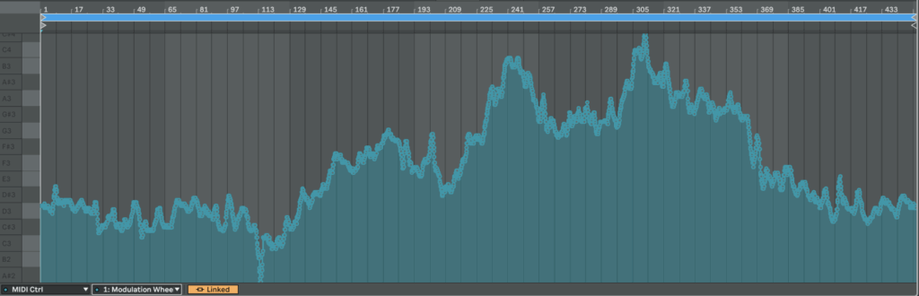
As a result, we get CC automation that we can easily map to something else or just copy automation somewhere else:
Here is an example of HR from patient 115 mapped from 0 to 127 in CC:
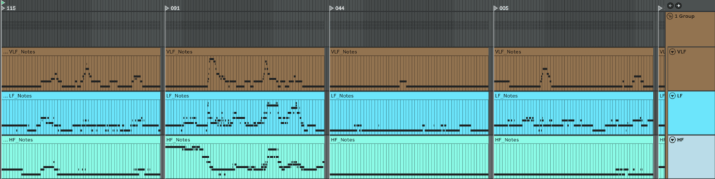
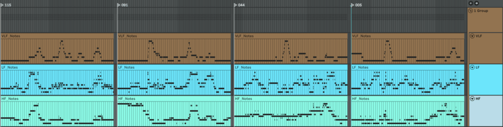
The next step after the drum generator is a harmonic layer built from frequency-domain HRV metrics. The script should do exactly what the drum code did for HR: scan all source files, find the global minima and maxima of every band, then map those values to pitches. Very-low-frequency (VLF) energy lives in the first octave, low-frequency (LF) in the second, high-frequency (HF) in the third. Each band is written to its own MIDI track so a different instrument can be assigned later, and every track also carries two automation curves: one CC lane for the band’s amplitude and one for the LF ⁄ HF ratio. In the synth that ratio will cross-fade between a sine and a saw: a large LF ⁄ HF—often a stress marker—makes the tone brighter and scratchier.
Instead of all twelve semitones, the script confines itself to the seven notes of C major or C minor. The mode flips in real time: if LF ⁄ HF drops below two the scale is major, above two it turns minor. Timing is flexible: each band can have its own step length and note duration so VLF moves more slowly than HF.
Below is a concise walk-through of ecg_to_notes.py. Key fragments of the code are shown inline for clarity. If you want to see the full, visit: https://github.com/ninaeba/EmbodiedResonance
# ----- core tempo & bar settings -----
DEF_BPM   = 75      # fixed song tempo
CSV_GRID  = 0.1     # raw data step in seconds
SIGNATURE = "8/8"   # eight cells per bar (fits VLF rhythms)
The script assigns a dedicated time grid, rhythmic value, and starting octave to each band. Those values are grouped in three parallel constants so you can retune the behaviour by editing one block.
Major and minor material is pre-baked as two simple interval lists. A helper translates any normalised value into a scale degree, then into an absolute MIDI pitch; another helper turns the same value into a velocity between 80 and 120 so you can hear amplitude without a compressor.
signals_to_midi opens one CSV, grabs the four relevant columns, and sets up three PrettyMIDI instruments—one per band. Inside a single loop the three arrays are processed identically, differing only in timing and octave. At each step the script decides whether we are in C major or C minor, converts the current value to a note and velocity, and appends the note to the respective instrument.
Every note time-stamp is paired with two controller messages: the first transmits the band amplitude, the second the LF / HF stress proxy. Both are normalised to the full 0-127 range so they can drive filters, wavetable morphs, or anything else in the synth.
The main wrapper gathers all CSVs in the chosen folder, computes global min–max values so every file shares the same mapping, and calls signals_to_midi on each source. Output files are named *_signals_notes.mid, each holding three melodic tracks plus two CC lanes per track. Together with the drum generator this completes the biometric groove: pulse drives rhythm, spectral power drives harmony, and continuous controllers keep the sound evolving.
Here is what we get if we make one mappinf for all patients
An here is example of MIDI files we get if we make individual mapping for each patient separetly
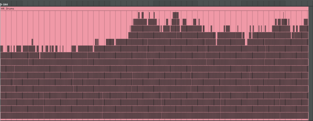
To generate heart-rate–driven drums I set out to write a script that builds a drum pattern whose density depends on HR intensity. I fixed the tempo at 75 BPM because the math is convenient: 0.1 s of data ≈ one 1/32-note at 75 BPM. I pictured a bar with 16 cells and designed a map that decides which cell gets filled next; the higher the HR, the more cells are activated. Before rendering, a helper scans the global HR minimum and maximum and slices that span into 16 equal zones (an 8-zone fallback is available) so the percussion always scales correctly. For extra flexibility, the script also writes SDNN and RMSSD into the MIDI file as two separate CC automation lanes. In Ableton, I can map those controllers to any parameter, making it easy to experiment with the track’s sonic texture.
This script converts raw heart-rate data into a drum track. Every 0.1-second CSV sample lines up with a 1⁄32-note at the fixed tempo of 75 BPM, so medical time falls neatly onto a musical grid. The pulse controls how many cells inside each 16-step bar are filled, while SDNN and RMSSD are embedded as two CC lanes for later sound-design tricks.
Default configuration (all constants live in one block)
 STEP_BEAT = 1 / 32  # grid resolution in beats
 NOTE_LENGTH = 1 / 32  # each hit lasts a 32nd-note
 DEF_BPM = 75    # master tempo
 CSV_GRID = 0.1   # CSV step in seconds
 SEC_PER_CELL = 0.1   # duration of one pattern cell
 SIGNATURE = "16/16" # one bar = 16 cells
 CC_SDNN = 11    # long-term HRV
 CC_RMSSD = 1    # short-term HRV
The spatial order of hits is defined by a map that spreads layers across the bar, so extra drums feel balanced instead of bunching at the start
generate_rules slices the global HR span into sixteen equal zones and binds each zone to one cell-and-note pair; the last rule catches any pulse above the top threshold
 def generate_rules(hr_min, hr_max, cells):
  thresholds = np.linspace(hr_min, hr_max, cells + 1)[1:]
  rules = [(thr, CELL_MAP[i], 36 + i) for i, thr in enumerate(thresholds)]
  rules[-1] = (np.inf, rules[-1][1], rules[-1][2])
  return rules
Inside csv_to_midi the script first writes two continuous-controller streams—one for SDNN, one for RMSSD—normalised to 0-127 at every grid tick
 sdnn_norm = clip((sdnn − min) / (range), 0, 1)
 rmssd_norm = clip((rmssd − min) / (range), 0, 1)
 add CC 11 with value round(sdnn_norm × 127) at time t
 add CC 1 with value round(rmssd_norm × 127) at time t
A cumulative-pattern list is built so rhythmic density rises without ever muting earlier layers
 CUM_PATTERNS = []
 acc = []
 for (thr, cell, note) in rules:
  acc.append((cell, note)) # keep previous hits
  CUM_PATTERNS.append(list(acc)) # zone n holds n+1 hits
During rendering each bar/cell slot is visited, the current HR is interpolated onto that exact moment, its zone is looked up, velocity is set to the rounded pulse value, and only the cells active in that zone fire
 hr = interp(t_sample, times, hr_vals)
 zone = first i where hr ≤ rules[i].threshold
 vel = int(round(hr))
for (z_cell, note) in CUM_PATTERNS[zone]: if z_cell ≠ cell: continue beat = (bar × cells + cell) × STEP_BEAT × 4 t0 = beat × 60 / bpm write Note(pitch=note, velocity=vel, start=t0, end=t0 + NOTE_LENGTH in seconds)
Before any writing starts the entry-point scans the whole folder to gather global minima and maxima for HR, SDNN and RMSSD, guaranteeing identical zone limits and CC scaling across every file in the batch
 hr_min, hr_max = min/max of all HR values
 sdnn_min, sdnn_max = min/max of all SDNN values
 rmssd_min, rmssd_max = min/max of all RMSSD values
 rules = generate_rules(hr_min, hr_max, cells)
Each CSV becomes a _drums.mid file that contains a single drum-kit track whose note density follows heart-rate zones and whose CC 11 and CC 1 envelopes mirror long- and short-term variability—ready to animate filters, reverbs or whatever you map them to in the DAW.
Here are examples of generated MIDI files with drums. On the left side, there are drums made with individual mapping for every patient separately, and on the right side, mapping is one for all patients. We can see they resemble our HR graphs.
In class, we did a rapid-fire round of 1-on-1 prototype testing. Each of us had about three minutes to present our prototype to a classmate, who would try to figure out how it works and what it represents, without much explanation.
My prototype was a small-scale physical room, just 10x10cm, constructed from paper. It had two vertical walls and a floor, with a “0” drawn on each of these surfaces to mark the starting point. From there, the interaction unfolded in layers.
The next components were two small paper strips, 1x3cm each. Folded in half and placed on top of the walls like little blades, these represented projectors. Then came two larger 10x10cm sheets, each marked with a “1” in the top left corner and colored pink. One of these was placed on the floor, the other on one of the walls. The pink floor piece had footprints drawn on it as signal of movement.
Finally, two more sheets were added this time green, labeled with a “2” and layered over the pink ones. On the green floor piece, small ripples of water replaced the original marks. Meanwhile the wall had raindrops in the same axis of the water ripples.
As classmates explored the prototype, the general response was encouraging. Many found it intuitive, the layering, the footprints, the shift from step to splash. However, the most consistent point of confusion was the tiny projector pieces. People weren’t sure what they were for, and in the fast-paced 3-minute window, that uncertainty took up valuable time.
This exercise reminded me how even small unclear elements can disrupt an otherwise understandable experience. But it also showed how much can be communicated through tactile storytelling. Overall, it was nice to see my idea come to life in others’ hands.
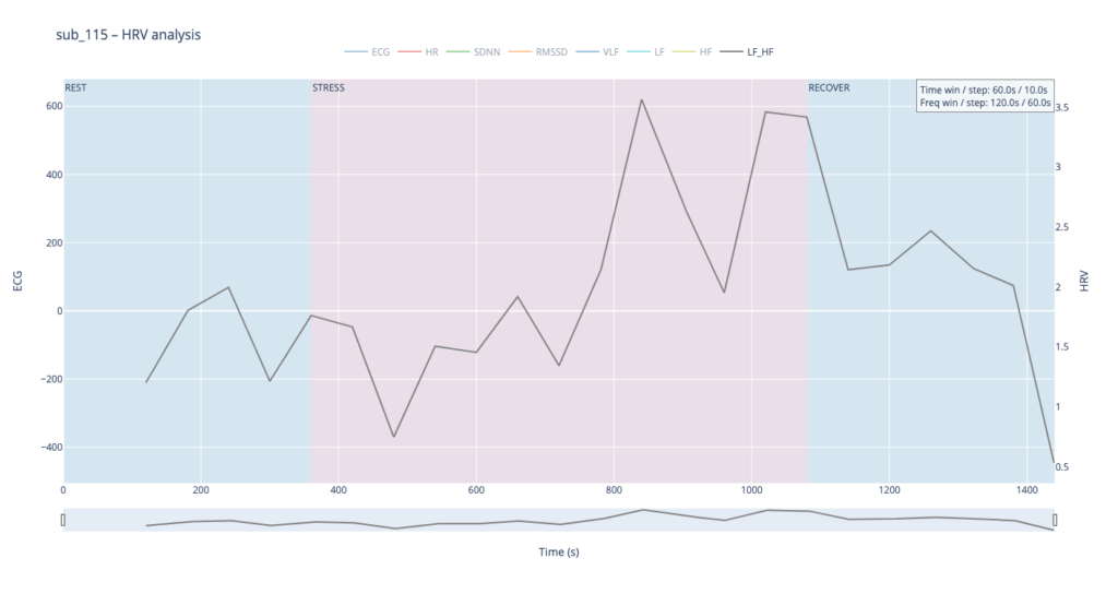
Below are the four participants whose heart-rate-variability traces we have explored. We deliberately chose them because they sit at clearly different points on the “health–illness” spectrum and therefore give us a compact but vivid physiological palette.
Subject 119 is our practical baseline. No cardiac findings, no anxiety-or-depression scores, no PTSD, no “Type-D” personality pattern. Anything we hear or see in this person’s HRV should approximate the dynamics of an uncomplicated, resilient autonomic system.
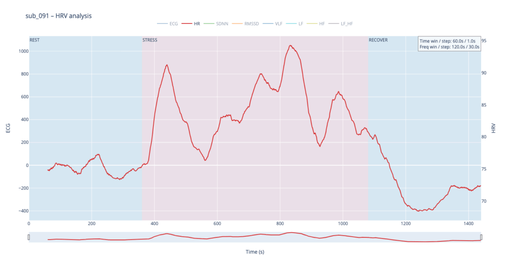
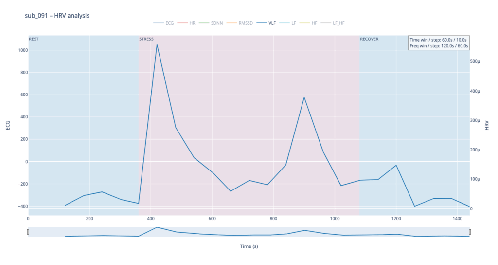
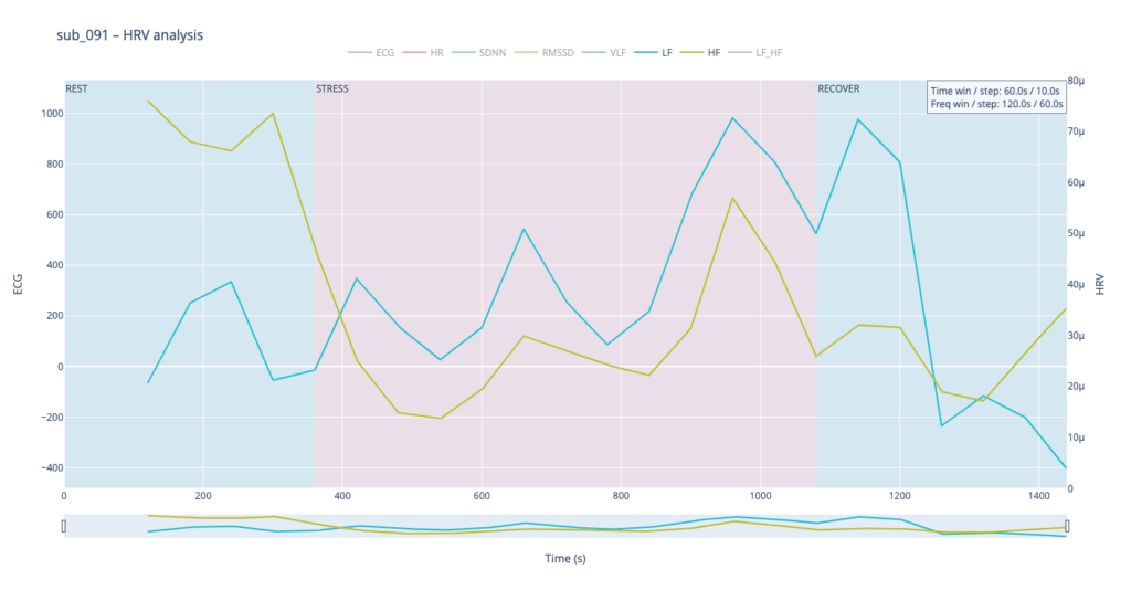
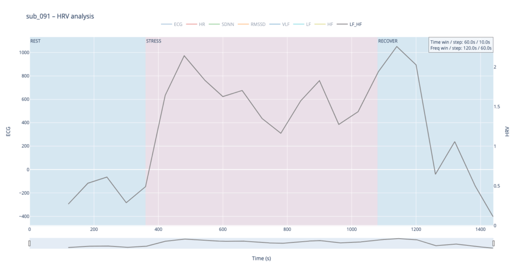
Subject 091 represents a “mind-only” disturbance. The heart itself is structurally sound, but the person carries the so-called Type-D trait (high negative affect, high social inhibition). This makes the autonomic system more reactive to worry or rumination even when the coronary vessels are normal.
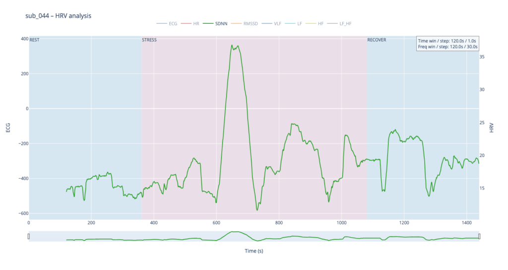
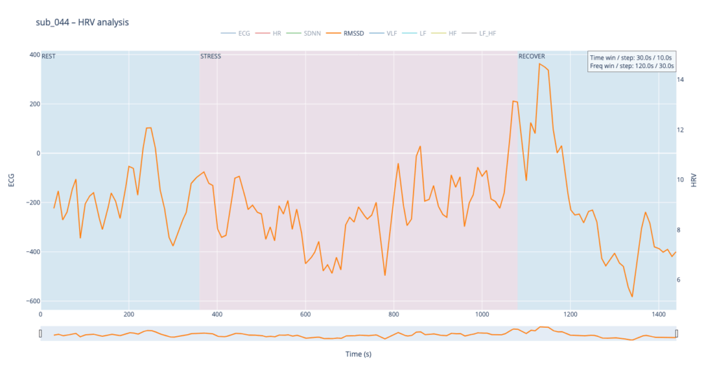
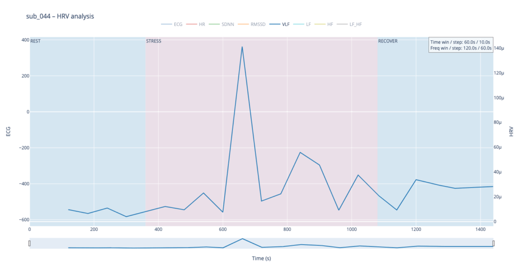
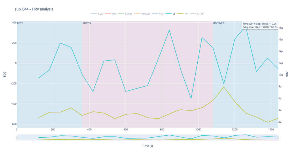
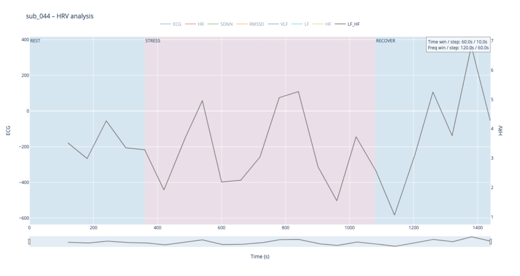
Subject 044 adds psychological trauma on top of mild, non-obstructive angina. Clinically this participant scores high on anxiety and meets full PTSD criteria. We therefore expect brisk sympathetic surges, slower vagal recovery and more noise in the LF/HF ratio—an autonomic pattern often seen in hyper-arousal states.
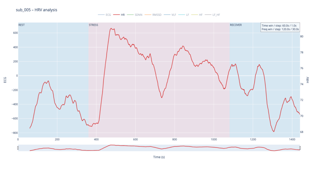
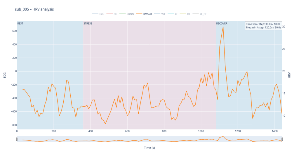
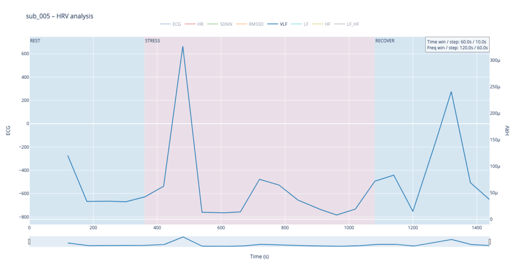
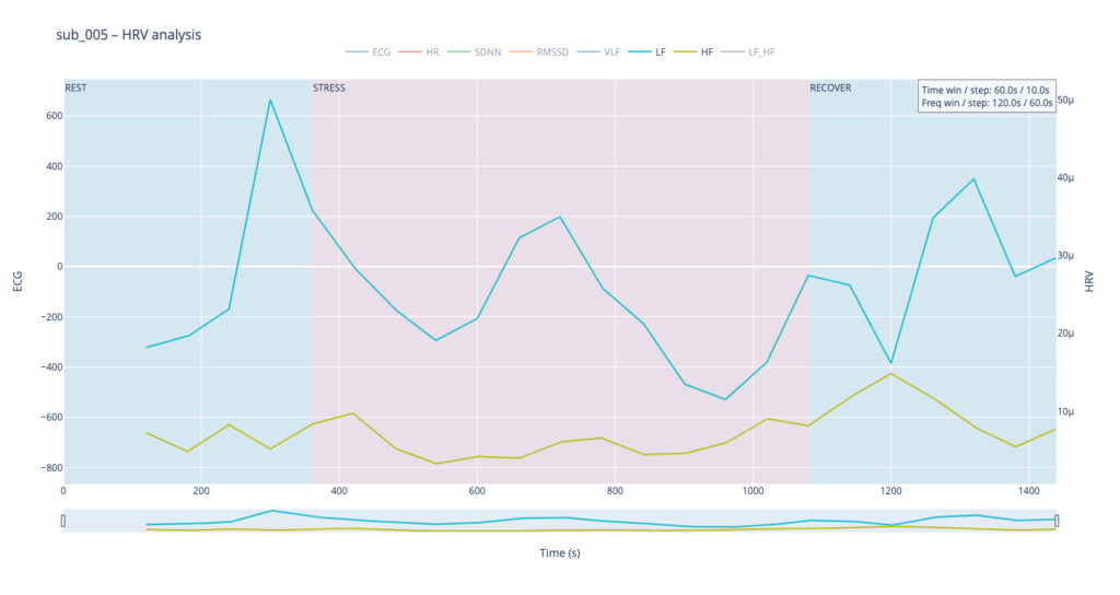
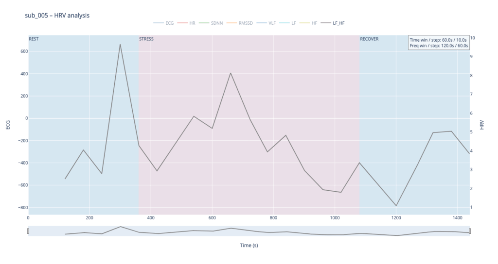
Subject 005 is the most medically burdened case: non-obstructive angina, endothelial dysfunction, stress-induced ischaemia, plus anxiety, depression, Type-D personality and PTSD. In short, both the mechanical pump and the emotional “software” are under strain, so variability measures are likely compressed and heart-rate plateaus may appear where a healthy person would fluctuate.
Using these four contrasting bodies as our “voices” lets us investigate how the same 6-min rest → 12-min exercise → 6-min recovery protocol is translated into four distinct autonomic narratives—information we will later map into equally distinct sonic textures.
HR
In general, each cardiovascular system answers physical load differently, depending on the baseline autonomic tone, fitness, psychological state, and comorbidities.
sub 115 – “healthy” The heart “ramps up” slowly. Pulse climbs in stair-like steps with brief dips between peaks—the body is constantly trying to regain homeostasis. After the exercise HR quickly falls almost to baseline. This is typical of a well-trained, adaptive cardiovascular system with a large functional reserve.
sub 091 – “mental / Type D” Resting HR is slightly above normal, yet overt anxiety is absent. The response is inertial: about a minute after load starts HR jumps from 75 → 91 bpm, then plummets to 76, followed by alternating short rises and falls. When the exercise stops, HR drops to 68 (below the initial value) and only then drifts back to ~75. Such a “swing” may reflect conflicting sympathetic vs. parasympathetic signals: outward calm while inner tension builds and discharges in bursts.
sub 044 – “PTSD” Even before load the heart is already in “fight-or-flight” mode (~83 bpm). The onset of exercise changes little, but at the third minute HR spikes to 98. It then declines stepwise yet remains high (89–97) even during recovery. The absence of a deep post-exercise dip shows that the parasympathetic “brake” hardly engages— the body struggles to shift into a resting state.
sub 005 – “sick / multiple pathologies” Baseline HR is 68. At the start of exercise it leaps to 80, after which it very slowly, step-by-step, drifts back toward normal and stays there until the end of the trial. The pattern resembles sub 044 but with lower background stress and slightly better recovery.
In healthy subjects the heart rate rises smoothly in step-like waves during effort and quickly settles back to baseline once the task stops, reflecting a well-balanced push-and-pull between sympathetic “accelerator” activity and parasympathetic (vagal) “brakes.” In patients with cardiac disease, PTSD or Type-D traits the resting rate is already elevated, the response to stress is sharper or more erratic, and the return to baseline is sluggish, showing a system locked in chronic “fight-or-flight” with weaker vagal damping.
Sound-design mapping:
Based on HR, I want to create drum patterns, where the lowest HR generates only kick, and then if HR rises, we can add more percusive elements.
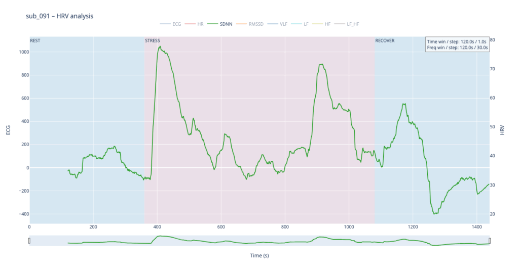
SDNN
SDNN tracks how much the RR-intervals expand and shrink over time.
When the value climbs, the spacing between beats becomes more irregular—your heart is “dancing” around the mean to satisfy moment-to-moment demands.
When the value sinks, the intervals line up almost like a metronome—either the organism is in very deep rest or the rhythm is held in a tight sympathetic “clamp” and cannot flex.
Usually this parameter is calculated for 24 hours, but since we dont have such luxury, we stick to 2min time window
Looking at all four traces, the healthy control shows the widest SDNN swing and more frequent surges during the load phase. This wide dynamic range tells us the cardiac pacemaker is quick to loosen and tighten the rhythm, i.e. it adapts smoothly to the body’s changing needs. By contrast, the clinical subjects operate in a narrower corridor: their SDNN rarely strays far from baseline, signalling that the heart either remains compressed by chronic sympathetic tone or cannot recruit enough parasympathetic “slack” to respond fully.
For the sound-mapping layer, I’d like to add a short delay on the Drums track and control athe mount of feedback and reverb of echoes.
RMSSD
RMSSD is conceptually close to SDNN, but it is calculated as the square root of the mean of the squared differences between successive RR intervals. In essence, RMSSD captures beat-to-beat (“breath-by-breath”) variability, whereas SDNN reflects overall dispersion of intervals within the chosen window. Because of this local focus, we processed RMSSD in a shorter analysis window—30 seconds with a 10-second step—to obtain a curve that is smooth yet sensitive to rapid changes.
The comparative analysis reveals patterns similar to SDNN, with several noteworthy differences. First, in the clinical subjects, the RMSSD range is almost twice as narrow, indicating reduced high-frequency variability—the heart is working in a more “rigid” mode. Second, in both pathological cases, RMSSD rises noticeably toward the end of the protocol: once exercise stops, sharp spikes appear that are virtually absent in the healthy subject. This delayed surge suggests a late engagement of parasympathetic control—the body remains under sympathetic drive for a prolonged period and only during recovery tries to compensate, generating erratic, uneven intervals.
To highlight the heart’s “rigidity,” I plan to map RMSSD to the pitch shift of drums.
Spectral HRV analysis
For spectral HRV analysis the gold-standard window is about five minutes, but in this project we need a compromise between scientific reliability and near-real-time responsiveness. We therefore use a 120-second window with a 60-second step.
VLF
Within such a short segment, the VLF band (0.003–0.04 Hz)—which is thought to reflect very slow regulatory processes such as hormonal release and thermoregulation—cannot be interpreted with the same statistical confidence as in traditional five-minute blocks. Even so, the plots still reveal that surges in VLF power tend to appear just before rises in heart-rate amplitude. In our context that timing may hint at micro-shifts in core temperature or other slow-acting homeostatic mechanisms that prime the cardiovascular system for the upcoming workload.
VLF → Sub-bass “body boil” layer We will map the slow-acting VLF band to a very low sub-bass drone in the first octave (≈ 30-60 Hz). As VLF power rises the pitch of this bass note is gently shifted upward by a few semitones and a subtle vibrato (slow LFO) is added. The result feels like liquid starting to simmer: higher VLF = hotter “water,” faster wobble, and a slightly higher fundamental. A pre-recorded low-frequency sample (e.g., pitched-down kettle rumble) can sit under the main mix; its playback pitch follows the same VLF curve to reinforce the sensation. When VLF falls, both pitch and vibrato relax, letting the bass settle back to its calm, foundational tone. This approach sonically frames VLF as the deep thermal undercurrent of the body.
LF & HF
Low-Frequency (LF, 0.04–0.15 Hz) and High-Frequency (HF, 0.15–0.40 Hz) power curves mirror the behavior we already saw with SDNN and RMSSD. That is perfectly logical: SDNN and LF both track activity of the sympathetic branch, which dominates under stress—heart rate accelerates, blood pressure rises, LF climbs. Conversely, HF and RMSSD follow the parasympathetic (“vagal”) branch: as the body relaxes, the heart slows, breathing deepens, and HF increases.
Patient 091 delivers a textbook illustration of that theory. At rest his HF overtops LF, but the moment exercise begins the autonomic balance flips—LF jumps above HF and keeps climbing, whereas HF rises more modestly and then drops back near the end, underscoring how hard it is for his system to settle.
By contrast, our other symptomatic patients (044 and 005) show LF dominating HF throughout, signalling a chronically tense autonomic state.
The healthy subject 115 starts with LF and HF almost equal; as effort mounts the gap widens in a smooth, orderly fashion.
Sonically, LF and HF make a natural complement to the VLF layer. We can map their absolute values to pitch in the second octave while using the LF/HF ratio to shape timbre—blending from a pure sine wave toward an edgier saw-like texture. When LF/HF is below 2, the sound stays near sine (calm, vagal tone); as the ratio exceeds 2, it becomes increasingly “saw-toothed,” evoking sympathetic arousal. Also, with this parameter, I would like to control the music scale from major to minor.
In practice, we see 115 and 091 resting in the neutral range and pushing upward only during exercise—the difference being that 115 ascends gradually, whereas 091 leaps. Both glide back to baseline once the task ends.
Patients 044 and 005, however, begin with ratios already high and jittering, telegraphing their persistent sympathetic load.
The next stage will be to develop an algorithm that converts these metrics into MIDI messages that can be mapped to parameters inside a DAW, or, alternatively, to build a SuperCollider or Pure Data patch implementing the same control scheme.