Tag: Sonification

The installation was presented on February 22 at ESC Medien Kunst Labor as part of the master’s exhibition “Overlays” (CMS, FH Joanneum).

To strengthen the conceptual layer of the work, I deliberately chose not to use headphones or conventional loudspeakers. Instead, I used two horn loudspeakers (model shown in the figures). Such speakers are commonly used in stadiums or public announcement systems and strongly resemble urban warning sirens. In addition to their visual reference, these speakers have very specific timbral characteristics: they do not reproduce frequencies below approximately 300 Hz and are highly directional, which significantly shaped the listening experience.

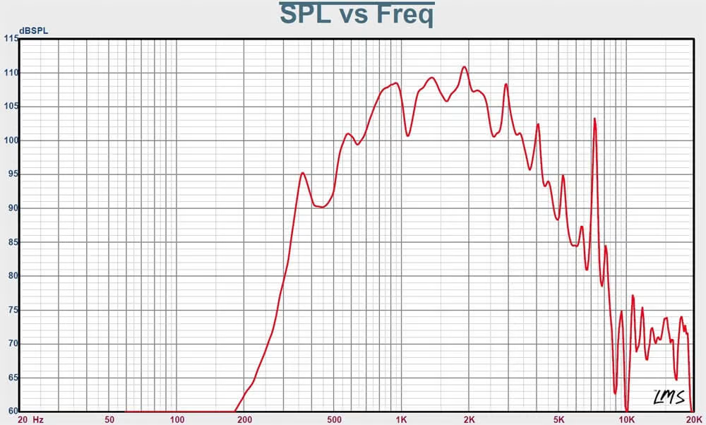
Frequency response (SPL vs. frequency) of the horn loudspeaker.

With the help of my supervisor Winfried Ritsch, who carefully calculated the required voltage, it was possible to safely connect the horn speakers to a standard OR.M CS-PA1 amplifier.

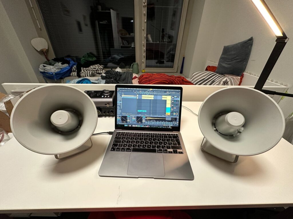
Test setup for horn loudspeakers during home prototyping.
https://dnh.no/products/hp-15t/ 

The speakers were suspended from the ceiling using metal chains attached to a metal truss structure, with a distance of approximately 120 cm between them. This spatial arrangement allowed visitors to physically enter the installation and stand between the speakers, experiencing the sound directly and bodily.

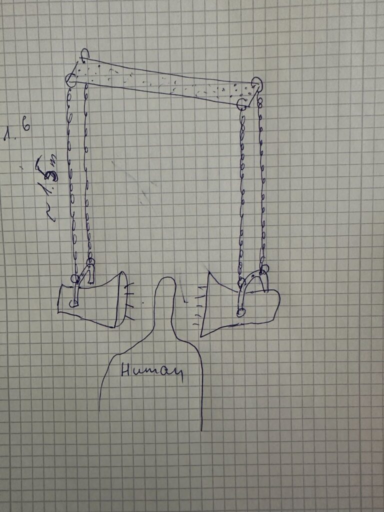
Installation layout sketches and spatial arrangement of sound sources and projection

The visual and spatial elements were arranged so that the light from a projector was directed toward the wall and the speakers in a way that their shadows became visible. The projected human silhouette was positioned between the shadows of the speakers, creating a layered visual composition that added a poetic and symbolic dimension to the installation.

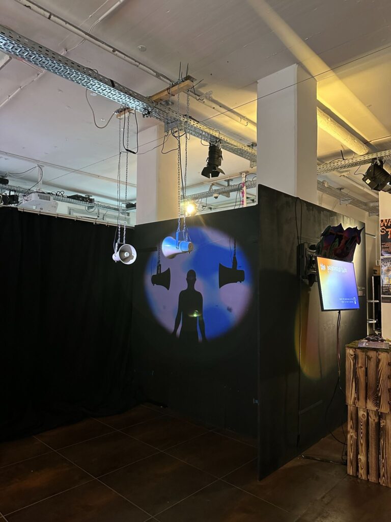
Installation in the exhibition space.

For playback, a simple media player was used, running a pre-rendered video file that already contained the synchronized audio. This decision significantly simplified the technical setup and ensured stable operation throughout the exhibition.

I would like to express special thanks to Gregor Schmitz, who assembled and installed the work. During the installation days, I was ill with influenza and had a high fever, which made it impossible for me to be physically present. Thanks to his persistence and careful work, the installation functioned reliably for the entire duration of the exhibition.

Conclusions

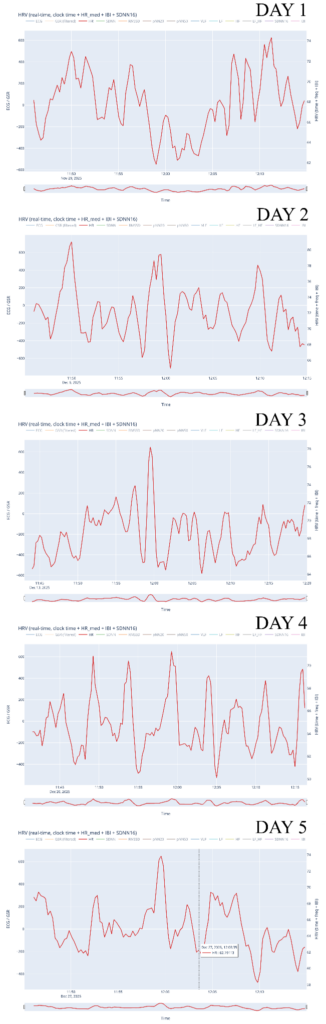
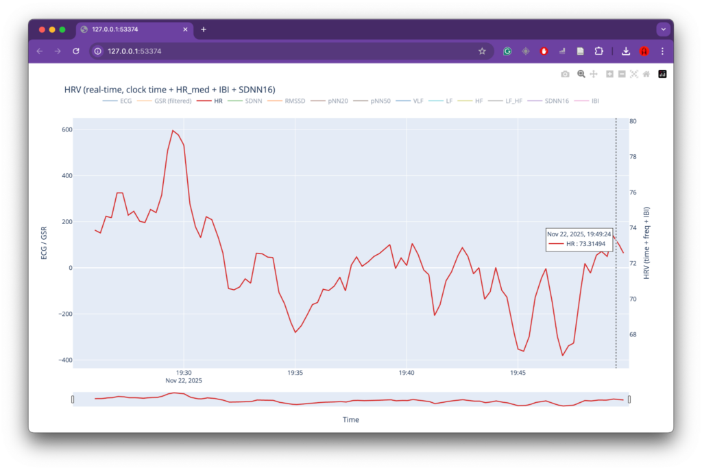
This project successfully combined physiological data analysis, sound design, and spatial installation into a coherent artistic system. One of its strongest aspects was the conceptual consistency between data, sound, and visual form. The use of HRV parameters as a driving force for both audio and visual processes created a clear and readable connection between bodily states and their artistic representation. The choice of horn speakers, their spatial placement, and their strong directional and timbral characteristics effectively reinforced the conceptual reference to sirens and public warning systems, adding both physical presence and symbolic weight to the installation. The decision to render audio and video together into a single media file also proved practical and reliable for exhibition conditions, significantly simplifying setup and playback.

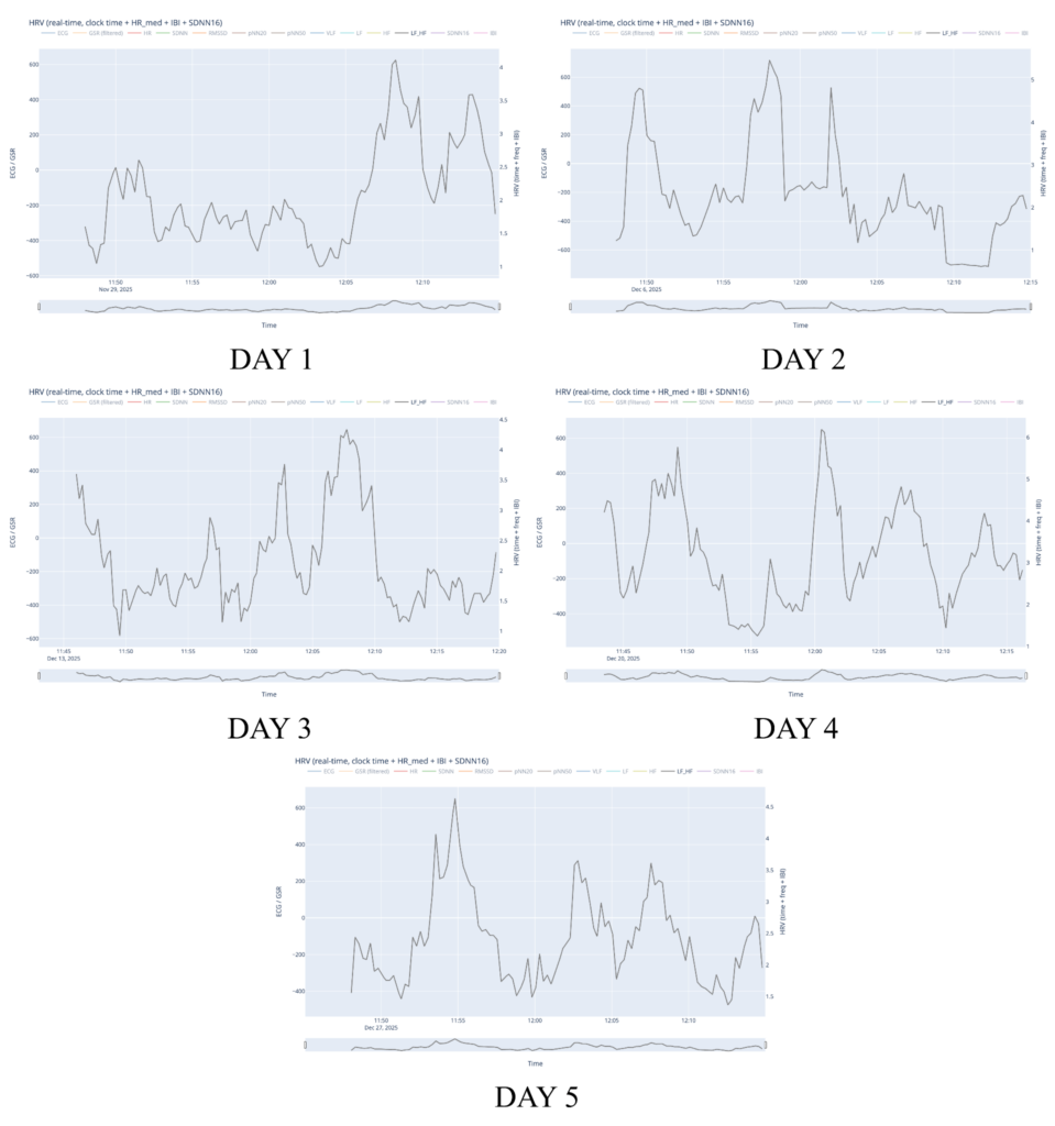
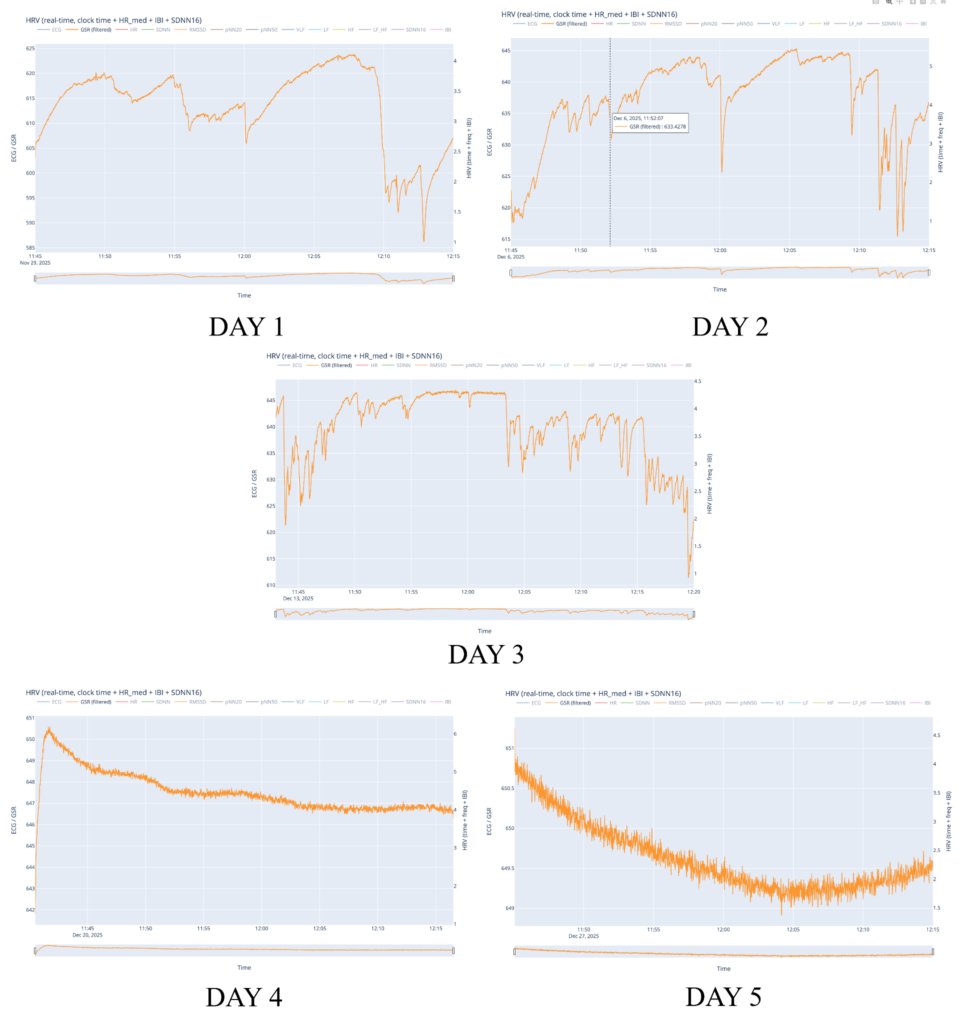
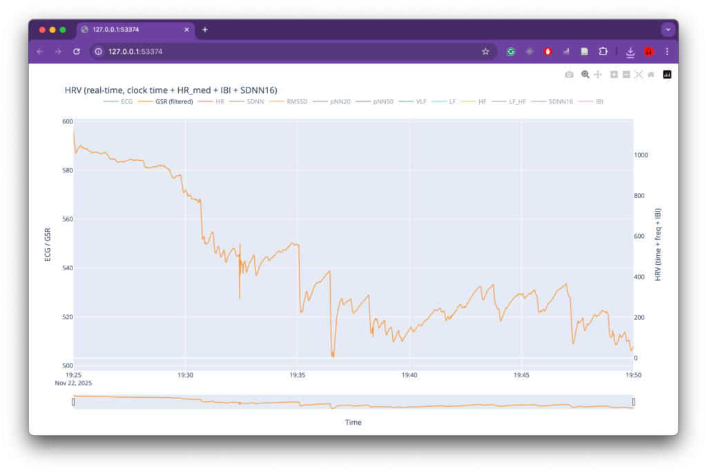
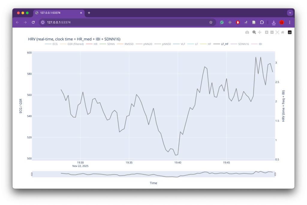
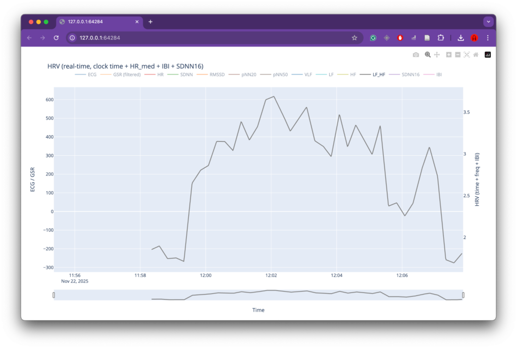
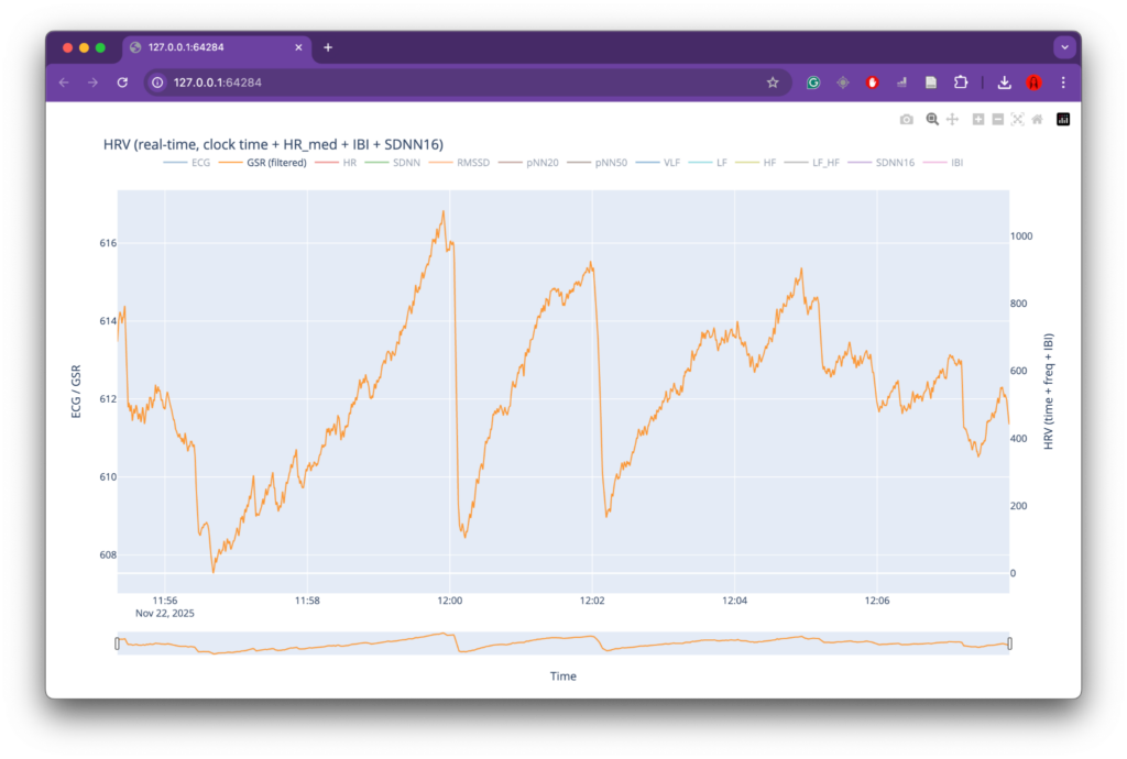
At the same time, several limitations became apparent, primarily related to data collection. While the overall data-processing and mapping workflow functioned as intended, the preparation phase for recording physiological data could have been more rigorous. The number of recordings was relatively limited, which reduced the robustness and representativeness of the dataset. In addition, recording conditions were not always fully controlled or stable, leading to inconsistencies and, in some cases, unusable data (such as the GSR measurements). These issues directly affected the range and reliability of parameters available for mapping and constrained the expressive potential of the system.

For future iterations, the most important improvement would be a more structured and controlled data-recording phase. This includes conducting a larger number of recordings, ensuring consistent environmental conditions, and clearly defining recording protocols in advance. More stable sensor placement, longer-term recordings, and repeated sessions under comparable conditions would significantly improve data quality and allow for deeper comparative analysis. With a more robust dataset, the mapping strategies could also be refined further, enabling more nuanced and complex relationships between physiological states, sound, and visuals. Overall, the project demonstrates strong artistic and technical foundations, while also clearly indicating directions for methodological refinement and expansion in future work.

During the preparation of the installation, I decided to extend the project with a visual layer that supports and reinforces the sound. The visual component was conceived as a minimal, data-driven system that mirrors the same physiological dynamics shaping the audio, rather than functioning as an independent narrative. For this purpose, I used TouchDesigner, where I created a relatively simple visual patch controlled by HRV-derived parameters. Instead of implementing real-time data streaming, I reused the MIDI files generated during the sound design stage. These MIDI signals were imported into TouchDesigner, normalized from the MIDI range (0–127) to values between 0 and 1, and used to drive visual modulation.

TouchDesigner patch for HRV-driven visual modulation.

The patch is structured around two parallel visual layers based on the same source footage: a video of the sky with birds flying through the frame. Each video layer undergoes a similar processing chain, including the addition of procedural noise, displacement, conversion to monochrome, and subsequent color mapping. 

As in the sound design, the two visual layers differ primarily in their color treatment. One layer is tinted in cool blue tones, while the other is dominated by red hues. Switching between these layers is controlled by the LF/HF ratio, which acts as a high-level indicator of autonomic balance. When the LF/HF value increases, corresponding to a stressed physiological state, the red-toned layer becomes dominant.

In addition to color changes, the patch applies displacement effects that are also influenced by HR. During moments of increased stress, the displacement intensity rises, causing the image to warp and fragment more strongly.

A human silhouette is layered on top of the background video. Under calm conditions, the silhouette remains stable and clearly defined. As stress increases, the silhouette becomes progressively distorted through displacement and noise-based modulation. This distortion visually emphasizes bodily tension and loss of internal stability, reinforcing the embodied dimension of the work.

After applying the HRV-to-CC conversion script, five MIDI files were generated—one for each recording day. A deliberate decision was made to normalize MIDI CC values (0–127) separately for each day rather than across the entire dataset. This approach emphasizes intra-day dynamics and allows relative physiological changes within a single session to be expressed more clearly through sound, rather than flattening them through global normalization.

MIDI CC automation derived from HR (CC1) and LF/HF (CC11).

In the conversion stage, specific MIDI CC numbers were preassigned to selected physiological parameters. Heart rate (HR) was mapped to MIDI CC 1 (Mod Wheel), and the LF/HF ratio was mapped to MIDI CC 11 (Expression). This choice was primarily practical: in Ableton Live, both CC 1 and CC 11 can be freely accessed and remapped using the Expression Control device, allowing flexible routing to multiple sound parameters without additional MIDI processing.

The core sound texture was constructed using a combination of Granulator II, Auto Pan (used in tremolo mode), Auto Filter, and Utility. Expression Control devices were used to distribute incoming MIDI CC data to multiple plugin parameters simultaneously.

The LF/HF ratio was used as a proxy for autonomic balance and stress level and was mapped to parameters that strongly affect spectral content and internal motion of the sound: Granulator II → Position, Grain Size, Variation
Auto Filter → Frequency, Resonance

Heart rate (HR) was mapped to parameters associated with rhythmic modulation, spatial perception, and perceived intensity:

Auto Pan →  Amount, Frequency

Granulator II →  Shape

Utility →  Stereo Width

Together, these mappings translate physiological arousal into changes in movement, brightness, density, and spatial spread of the sound texture.

In parallel, a second, identical processing chain was created using the same plugin structure but a different sound source and an inverted mapping strategy. The two granular layers were combined inside an Instrument Rack, preceded by an additional Expression Control device.

Overview of the mapping between HRV parameters, MIDI CC signals, and audio processing parameters.

The two sound sources used were:

Layer 1: an airy pad sample with subtle vinyl noise and bird sounds

Layer 2: a field recording of an air-raid siren from Kyiv

The LF/HF ratio was additionally mapped to the Chain Selector of the Instrument Rack, enabling a continuous crossfade between the two layers:

Low LF/HF values → dominance of the pad and bird sounds

High LF/HF values → dominance of the siren texture

As a result, the overall sound gradually shifts toward a siren-like timbre during periods of elevated physiological stress, and toward a softer, atmospheric texture during calmer states. Rather than triggering discrete sound events, this approach produces a continuously evolving audio texture that reflects internal physiological dynamics over time.

During HRV computation, all extracted parameters are stored in a new CSV file, with one row per time step. Building on the experiments conducted in the previous semester, a dedicated conversion script was developed to translate these HRV parameters into MIDI continuous controller (CC) signals for use in sound synthesis and composition.

The conversion process is based on three core principles. First, all physiological parameters are represented as independent CC lanes, allowing each metric to modulate a different sound parameter in a digital audio workstation. Heart rate is exported both as a raw value (clamped to the MIDI range 0–127) and as a normalized value scaled across the full CC range using global minimum and maximum values. This dual representation enables flexible artistic use of absolute and relative changes in heart rate.

Second, the script applies time compression to the physiological data. Because HRV parameters evolve slowly, real recording time is compressed so that long physiological processes can be perceived within a shorter musical timeframe. For example, several minutes of HRV data can be mapped onto a few seconds of MIDI time, while maintaining the temporal relationships between parameters. The compression factor can be adjusted depending on the desired level of temporal abstraction.

Third, normalization is performed using global minimum and maximum values computed across all available HRV CSV files. This ensures consistent scaling between different recording sessions and prevents abrupt changes in mapping behavior when multiple datasets are combined within the same composition.

For each time step in the HRV CSV file, the script generates a group of MIDI CC messages that occur simultaneously. Each HRV parameter is linearly mapped to the MIDI range of 0–127 and written as a CC event at a fixed musical tempo. The resulting MIDI files therefore encode physiological dynamics as continuous control data, independent of note events.

This approach produces MIDI files that are immediately usable in digital audio workstations such as Ableton Live. HRV-derived CC lanes can be assigned to synthesis, filtering, spatialization, or effect parameters, forming a direct bridge between physiological analysis and sound-based artistic exploration.

Following the initial experiments, ECG and GSR recordings were conducted consistently over a period of five weeks during the weekly civil defense siren tests on Saturdays. Each recording session typically began between 11:30 and 11:40, allowing sufficient time to later remove several minutes of motion-related noise caused by movement, setup, and settling into a stable posture for recording.

It is important to note that I generally follow a late chronotype (“night owl”) sleep pattern and tend to wake up relatively late, especially on weekends. As a result, during most Saturday siren tests I was still in bed. Rather than attempting to alter this routine, I deliberately chose to maintain it in order to preserve ecological validity. All recordings were therefore conducted in bed, under a blanket, in a resting position consistent with a typical weekend morning. Although these Saturdays were dedicated to working on the project, the physical and contextual conditions were intentionally kept as close as possible to a habitual state.

I usually woke up around 11:00, completed the necessary preparations, and often attempted to set up the recording equipment on Friday evening to reduce time pressure. After attaching the ECG electrodes, I returned to bed and waited for the siren, keeping the window slightly open to ensure that the sound was clearly audible. For analysis, each recording was trimmed to retain approximately 15 minutes before and 15 minutes after the siren onset. The resulting segments were then processed using the established analysis pipeline.

Contrary to the initial hypothesis, the results of these repeated recordings did not show a consistent or clearly separable heart rate response before and after the siren. In particular, heart rate values were often already elevated at the beginning of the recording, prior to the siren onset. A plausible explanation for this pattern is the experimental context itself. On the nights preceding the recordings, I frequently went to bed late and woke up insufficiently rested. In addition, there was often time pressure in the morning to complete setup before the siren at 11:45. As a result, a heightened physiological arousal state was likely present already at the start of the experiment.

In several sessions (notably days 3 and 5), heart rate began to rise even before the siren, suggesting an anticipatory stress response associated with waiting for the event rather than reacting to the sound itself.

The LF/HF ratio provided slightly clearer indications of stress-related changes, although with considerable variability. On the first recording day, LF/HF showed a pronounced increase after the siren. On the second day, however, the behavior of this metric differed substantially. During days 3, 4, and 5, a tendency toward increased LF/HF after the siren was often observable, but in several cases the increase began before the siren, again suggesting a pre-existing stress state of the autonomic nervous system.

LF/HF  from five weekly siren test sessions.

The only parameter that behaved consistently across sessions was the GSR signal. Each time the siren sounded, a sharp drop in GSR values was observed. However, for reasons that remain unclear, the sensor did not function correctly during the final two recording sessions. The recorded GSR data from these sessions did not reflect plausible physiological responses and were therefore considered unreliable. As a result, GSR could not be used further as a parameter for sound mapping.

GSR  from five weekly siren test sessions.

Rather than discarding these recordings as unreliable, I chose to accept the limitations and realities of the experimental conditions. The longitudinal dataset is therefore approached not as a controlled physiological study, but as a form of embodied, self-reflexive investigation. The recordings capture a body shaped by multiple interacting factors—sleep, anticipation, routine, and personal history—and reflect the complexity of measuring stress responses in real-life contexts rather than laboratory environments.

In addition to the siren test recording, a further exploratory experiment was conducted later the same day under controlled indoor conditions. The aim of this session was to observe physiological responses to a pre-designed auditory scenario resembling elements of an air-raid situation, while maintaining full control over timing and sound structure.

Prior to the experiment, a long-form audio file was prepared. The recording began with ten minutes of continuous rain sounds. At the ten-minute mark, a civil defense siren was introduced, followed approximately one and a half minutes later by an explosion sound. The siren–explosion sequence lasted for three minutes and gradually faded out. Throughout this phase, the rain sound remained present and continued for an additional twelve minutes after the end of the siren and explosion. The experiment started at 19:25 and ended at approximately 19:50. All sound materials were sourced from soundfree.org and consisted of field recordings made in Kyiv.

Ableton Live session showing the audio structure used in the experiment (rain, siren, and explosion sounds).

The heart rate response during this experiment revealed several notable features. The first pronounced increase in heart rate occurred shortly before 19:30. At this moment, no siren or explosion had yet been played. Instead, this increase coincided with anticipatory thoughts related to the upcoming sounds, specifically concerns about playback volume and the potential intensity of the explosion sound. After briefly adjusting the volume and returning to a resting position, heart rate gradually decreased. However, with the onset of the siren and subsequent explosion sounds, heart rate increased again. This pattern suggests that not only the auditory stimulus itself, but also the anticipation of an expected threat-related sound, can activate a physiological fight-or-flight response.

Heart rate during the audio-based experiment. 

Consistent with the previous recording, the GSR signal showed rapid and pronounced changes. Sharp drops in GSR values were observed at the onset of the siren and again approximately one and a half minutes later, coinciding with the explosion sound. These abrupt responses indicate that skin conductance reacts very quickly to sudden or salient auditory events, often preceding slower cardiovascular changes.

GSR signal during the audio-based experiment.

The LF/HF ratio behaved in a less predictable manner during this experiment. Changes in LF/HF occurred more gradually and, notably, the ratio decreased following the end of the siren–explosion sequence. After this decrease, LF/HF values began to rise strongly during the later phase of the recording. Due to the complexity of this pattern and the limited number of repetitions, no clear interpretation could be drawn at this stage.

LF/HF during the audio-based experiment.

This experiment was conducted only once, and the subjective experience was described as unpleasant. In retrospect, the use of rain sounds both before and after the siren and explosion may have introduced a confounding factor, as rain is generally associated with calming effects. For this reason, the results of this experiment should not be used as a primary basis for quantitative analysis. Nevertheless, the recording remains qualitatively informative, particularly in demonstrating the role of anticipation and the differing temporal dynamics of cardiovascular and skin conductance responses.