Product V – Embodied Resonance – Initial Test Recording and Data Analysis

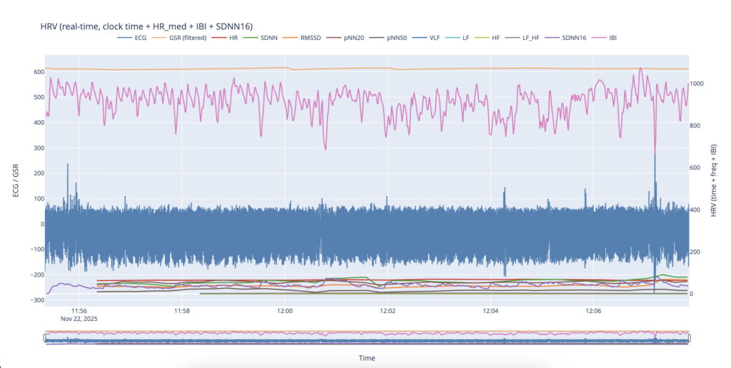
The first test recording during a civil defense siren was conducted on November 22. Data acquisition started at approximately 11:52. In retrospect, the recording was initiated too late, which significantly limited its analytical value. As a result, this dataset could not be used for systematic comparison between pre-siren and post-siren phases. Nevertheless, it served as a functional test of the recording and analysis pipeline. Additionally, the raw recording contained substantial motion-related noise at both the beginning and the end of the session. Approximately the first three minutes of the recording were removed during preprocessing, as the signal quality in this segment was insufficient for reliable analysis. Despite these limitations, the remaining portion of the recording provided useful preliminary insights.

Even in this shortened test recording, several initial assumptions were supported by the data. The most immediately noticeable change was a rapid increase in heart rate following the onset of the siren at 12:00. This abrupt rise suggests an acute physiological response triggered by the siren signal.

Heart rate response during the initial test recording.

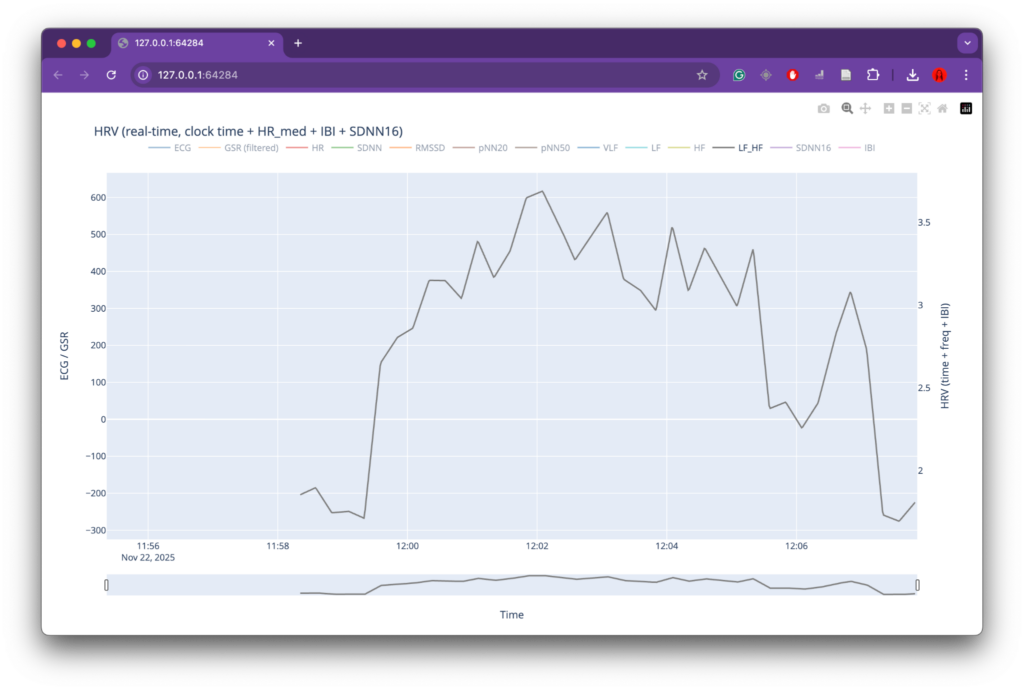
LF/HF ratio during the initial test recording.

A similar pattern was observed in the LF/HF ratio. The increase in this metric following the siren onset is commonly interpreted as a shift toward sympathetic nervous system dominance, which is associated with stress and heightened arousal. Although this observation aligns with the working hypothesis that the siren acts as a stressor for a person with lived experience of war, the short duration of the recording and the absence of a clear baseline phase prevent any strong conclusions at this stage.

The behavior of the GSR signal was particularly striking. At the moment the siren began, the GSR signal showed a sharp drop in values, indicating a rapid change in skin conductance. This response occurred faster than the corresponding changes observed in heart rate–related measures. Such behavior is consistent with the role of skin conductance as a fast-reacting indicator of autonomic arousal and attentional activation. Civil defense sirens are explicitly designed to capture attention, and the immediacy of the GSR response may reflect this design principle. Similar abrupt drops were visible later in the recording; however, due to the limited contextual information and short recording window, their exact causes could not be clearly identified.

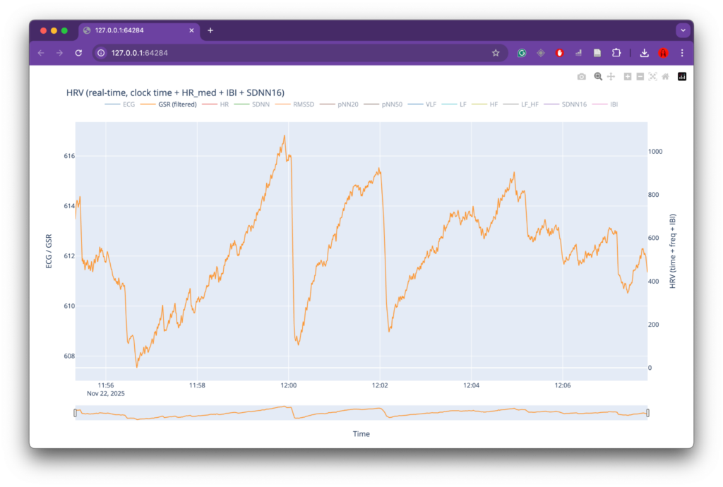
GSR signal over time during the initial test recording.

Other computed HRV metrics did not show clear or interpretable changes in relation to the siren onset within this test recording. For this reason, these parameters were not analyzed in depth at this stage and were deprioritized in subsequent analyses.

Overall, this first test recording confirmed the technical viability of the system and provided early qualitative support for the project’s core hypothesis. At the same time, it highlighted the need for longer recordings with clearly defined baseline periods and reduced motion artifacts, which informed the design of subsequent data acquisition sessions.

Product IV – Embodied Resonance – Signal Visualization and Analysis Tool

For signal inspection and analysis, I extended the Plotly-based ECG and HRV visualization tool developed during the previous semester. While the earlier version functioned well for simulated or pre-structured datasets, several adjustments were required to accommodate the properties of the new Arduino-based recordings.

The first challenge concerned the sampling rate. Unlike laboratory datasets with a fixed sampling frequency, the Arduino-based ECG stream does not produce perfectly uniform time intervals between samples. To address this, the analysis pipeline was adapted to work with a variable sampling rate derived from recorded timestamps rather than assuming a constant value. The effective sampling frequency is estimated from the median difference between successive time samples, which provides a robust approximation suitable for filtering and peak detection.

The second major modification involved time representation on the x-axis. In the previous implementation, signals were plotted against sample indices. In the current version, the visualization uses real recording time, allowing ECG, GSR, and derived HRV metrics to be aligned with the actual temporal structure of the experiment. 

A third extension was the integration of the GSR signal into the plotting and analysis pipeline. Due to the high noise level observed in the raw GSR signal, basic low-pass filtering was introduced to suppress high-frequency fluctuations and improve interpretability.

Later, beyond raw signal visualization, several additional heart rate variability metrics were implemented. In addition to standard time-domain measures such as SDNN and RMSSD, the analysis includes inter-beat intervals (IBI), which represent the temporal distance between successive R-peaks. IBI is closely related to respiratory modulation of heart rate and served as an important conceptual reference, inspired by the RESonance biofeedback experiment.

Following this inspiration, SDNN16 was added as a short-term variability metric that updates continuously with each detected heartbeat. Unlike conventional SDNN, which requires longer time windows, SDNN16 provides a fast-responding measure of variability that is well suited for dynamic visualization and potential sound mapping.

Furthermore, the metrics pNN20 and pNN50 were implemented. These parameters quantify the percentage of successive beat-to-beat interval differences exceeding 20 ms and 50 ms, respectively. Both metrics offer additional insight into short-term fluctuations in heart rhythm and were included as potential control parameters for later stages of sonification.

Together, these modifications resulted in a visualization and analysis tool capable of handling irregularly sampled data, aligning physiological signals with real recording time, and providing an expanded set of HRV descriptors. 

Product III – Embodied Resonance – Data Logging via Serial Communication

A custom Python script was developed to record ECG and GSR data streamed from the Arduino via the serial interface. The Arduino transmits raw sensor values as comma-separated integers (ECG, GSR) at a fixed baud rate. On the computer side, the Python script establishes a serial connection, continuously reads incoming data, and stores it in a structured CSV file together with precise timing information. 

Serial connection and configuration

PORT = “/dev/tty.usbmodem1101”

BAUD = 115200

ser = serial.Serial(PORT, BAUD)

This section defines the serial port and baud rate used by the Arduino. The baud rate must match the value specified in the Arduino sketch to ensure correct data transmission.

Automatic file creation and session-based storage

start_stamp = datetime.now().strftime(“%Y%m%d_%H%M%S”)

csv_filename = f”{start_stamp}_ecg_gsr.csv”

Each recording session generates a new CSV file whose name includes a timestamp. This prevents accidental overwriting and allows recordings to be clearly associated with specific experimental sessions.

CSV structure and timing

writer.writerow([“timestamp”, “time_ms”, “ECG”, “GSR”])

start_time = time.time()

The CSV file contains both an absolute timestamp and a relative time counter in milliseconds. This dual timing system supports synchronization with experimental events while also enabling precise signal processing.

Parsing and writing incoming data

line = ser.readline().decode(errors=”ignore”).strip()

ecg_str, gsr_str = line.split(“,”)

ecg = int(ecg_str)

gsr = int(gsr_str)

Each line received from the serial port is expected to contain two comma-separated values. Basic validation ensures that malformed or incomplete lines are ignored.

Writing samples to CSV

time_ms = int((time.time() – start_time) * 1000)

timestamp = datetime.now().strftime(“%Y-%m-%d %H:%M:%S.%f”)[:-3]

writer.writerow([timestamp, time_ms, ecg, gsr])

For each valid sample, the script writes one row containing the current timestamp, elapsed time since the start of recording, and raw ECG and GSR values. Data is flushed to disk continuously to prevent loss during longer sessions.

Product XI: Image Extender

From Notebook Prototype to Local, Exhibitable Software

This iteration was less about adding new conceptual capabilities and more about solidifying the system as an actual, deployable artifact. The core task was migrating the image extender from its experimental form into a standalone local application. What sounds like a technical refactor turned out to be a decisive shift in how the system is meant to exist, be used, and be encountered.

Until now, the notebook environment functioned as a kind of protected laboratory. It encouraged rapid iteration, verbose configuration, and exploratory branching. Moving out of that space meant confronting a different question: what does this system look like when it stops being a research sketch and starts behaving like software?

The transition from Colab-style execution to a locally running script forced a re-evaluation of assumptions that notebooks quietly hide:

  • Implicit state becomes explicit
  • Execution order must be deterministic
  • Errors can no longer be “scrolled past”
  • Configuration must be intentional, not convenient

Porting the logic meant flattening the notebook’s narrative structure into a single, readable execution flow. Cells that once assumed context had to be restructured into functions, initialization stages, and clearly defined entry points. This wasn’t just cleanup, it was an architectural clarification.

In the notebook, ambiguity is tolerated. In running software, it accumulates as friction.

Reduction as Design: Cutting Options to Increase Clarity

One of the more deliberate changes during this phase was a reduction in exposed settings. The notebook version allowed extensive tweaking, model switches, resolution variants, prompt behaviors, fallback paths, all useful during development, but overwhelming in a public-facing context.

For the exhibition version, optionality became noise.

Instead of presenting the system as a configurable toolkit, I reframed it as a guided instrument. Core behaviors remain intact, but the number of visible parameters was intentionally constrained. This aligns with a recurring principle in the project: flexibility should live inside the system, not on its surface.

Adapting for Exhibition: Y2K as Interface Language

Alongside the structural changes, the interface was visually adapted to match the exhibition context. The decision to lean into a Y2K-inspired color palette wasn’t purely aesthetic; it functioned as a form of contextual grounding.

The visual layer needed to communicate that this is not a neutral utility, but a situated artifact. The Y2K styling introduced:

  • High-contrast synthetic colors
  • Clear visual hierarchy
  • A subtle nod to early digital optimism and machinic playfulness

Rather than competing with the system’s conceptual weight, the styling makes its artificiality explicit.

Stability Over Novelty

Another quiet but important shift was prioritizing stability over feature expansion. The migration process exposed several edge cases that were easy to ignore in a notebook but unacceptable in a live context: silent failures, unclear loading states, brittle dependencies.

Addressing these didn’t add visible functionality, but they fundamentally changed how trustworthy the system feels. In an exhibition setting, reliability is part of the experience. A system that hesitates or crashes invites interpretation for the wrong reasons.

Here, robustness became a form of authorship.

Reframing the System’s Status

By the end of this iteration, the most significant change wasn’t technical, it was ontological. The system is no longer best described as “a notebook that does something interesting.” It is now a runnable, bounded piece of software, designed to be encountered without explanation.

This transition marks a subtle but important moment in the project’s lifecycle:

  • From private exploration to public behavior
  • From configurable experiment to opinionated instrument
  • From development environment to exhibited system

The constraints introduced in this phase don’t limit future growth, they define a stable core from which growth can happen meaningfully.

If earlier updates were about expanding the system’s conceptual reach, this one was about giving it a body.

Product X: Image Extender

Extending the System from Image Interpretation to Image Synthesis

This update marked a conceptual shift in the system’s scope: until now, images functioned purely as inputs, sources of visual information to be analyzed, interpreted, and mapped onto sound. With this iteration, I expanded the system to also support image generation, enabling users not only to upload visual material but to synthesize it directly within the same creative loop.

The goal was not to bolt on image generation as a novelty feature, but to integrate it in a way that respects the system’s broader design philosophy: user intent first, semantic coherence second, and automation as a supportive, not dominant, layer.

Architectural Separation: Reasoning vs. Rendering

A key early decision was to separate prompt reasoning from image rendering. Rather than sending raw user input directly to the image model, I introduced a two-stage pipeline:

  1. Prompt Interpretation & Enrichment (GPT-4.1)
    Responsible for understanding vague or underspecified user prompts and rewriting them into a semantically complete, realistic scene description.
  2. Image Synthesis (gpt-image-1 → DALL-E 2/3)
    Dedicated purely to rendering the final image from the enriched prompt. Through implementation, I discovered that while the original spec referenced gpt-image-1, OpenAI’s actual models are DALL-E 2 (60% cheaper, faster, but less detailed) and DALL-E 3 (higher quality but more expensive).

This separation mirrors the system’s audio architecture, where semantic interpretation and signal processing are deliberately decoupled. GPT-4.1 acts as a semantic mediator, while the image model remains a deterministic renderer.

The Response Format Learning Curve

During implementation, I encountered a subtle but important API nuance that forced a deeper understanding of the system’s data flow: DALL-E models return URLs by default, not base64 data. The initial implementation failed with a confusing “NoneType” error because I was trying to decode a base64 field that didn’t exist.

The fix was elegantly simple, adding response_format=”b64_json” to the API call—but the debugging process revealed something more fundamental about API design: different services have different default behaviors, and understanding those defaults is crucial for robust system integration.

This also led to implementing proper fallback logic: if base64 isn’t available, the system gracefully falls back to downloading from the image URL, ensuring reliability across different OpenAI model versions and configurations.

Interactive Workflow Integration with Toggle Architecture

To maintain consistency with the existing interactive toolset while adding flexibility, I implemented a mode-toggle architecture:

  • Upload Mode: Traditional file upload with drag-and-drop support
  • Generate Mode: Text-to-image synthesis with prompt enrichment
  • State Preservation: The system maintains a single IMAGE_FILE variable that can be overwritten by either mode, ensuring seamless transitions between workflows

The interface exposes this through clean toggle buttons, showing only the relevant UI for each mode. This reduces cognitive load while preserving full functionality, a principle I’ve maintained throughout the system’s evolution.

Cost-Aware Design with Caching and Model Selection

Image synthesis presents unique cost challenges compared to text generation or audio processing. I implemented several cost-mitigation strategies learned through experimentation:

  1. Resolution Control: Defaulting to 1024×1024  or 512×512 (for DALL-E 2)
  2. Quality Parameter Awareness: Only DALL-E 3 supports quality=”standard” vs “hd”—using the wrong parameter with DALL-E 2 causes API errors

The cost considerations weren’t just about saving money—they were about enabling iteration. When artists can generate dozens of variations without financial anxiety, they explore more freely. The system defaults to the cheapest viable path, with quality controls available but not forced.

Prompt Realism as a Soft Constraint

Rather than enforcing hard validation rules (e.g., predefined lists of places or objects), I chose to treat realism as a soft constraint enforced by language, not logic.

User prompts are passed through a prompt-enrichment step where GPT-4.1 is instructed to:

  • Reframe the input as a photographic scene
  • Ensure the presence of spatial context (location, environment)
  • Ground the description in physical objects and lighting
  • Explicitly avoid illustrated, cartoon, or painterly styles

This approach preserves creative freedom while ensuring that the downstream image generation remains visually coherent and photo-realistic. Importantly, the system does not reject user input—it interprets it.

Design Philosophy: Generation as a First-Class Input

What this update ultimately enabled is a shift in how the system can be used:

  • Images are no longer just analyzed artifacts
  • They can now be constructed, refined, and immediately fed into downstream processes (visual analysis, audio mapping, spatial inference)

This closes a loop that previously required external tools. The system now supports a full cycle: imagine → generate → interpret → sonify.

Crucially, the same principle that guided earlier updates still applies: automation should amplify intent, not replace it. Image generation here is not about producing spectacle, but about giving users a controlled, semantically grounded way to define the visual worlds their soundscapes respond to.

The implementation journeyfrom API quirks to cost optimization to user experience design, reinforced that even “simple” features require deep consideration when integrating into a complex creative system. Each new capability should feel like it was always there, waiting to be discovered.

Product IX: Image Extender

Moving Beyond Dry Audio to Spatially Intelligent Soundscapes

My primary objective for this update was to bridge a critical perceptual gap in the system: while the previous iterations successfully mapped visual information to sonic elements with precise panning and temporal placement, the resulting audio mix remained perceptually “dry” and disconnected from the image’s implied acoustic environment. This update introduces adaptive reverberation, not as a cosmetic effect, but as a semantically grounded spatialization layer that transforms discrete sound objects into a coherent, immersive acoustic scene.

System Architecture

The existing interactive DAW interface, with its per-track volume controls, sound replacement engine, and user feedback mechanisms, was extended with a comprehensive spatial audio processing module. This module interprets the reverb parameters derived from image analysis (room detection, size estimation, material damping, and spatial width) and provides interactive control over their application.

Global Parameter State & Data Flow Integration

A crucial architectural challenge was maintaining separation between the raw audio mix (user-adjustable volume levels) and the reverb-processed version. I implemented a dual-state system with:

  • current_mix_raw: The continuously updated sum of all audio tracks with current volume slider adjustments.
  • current_mix_with_reverb: A cached, processed version with reverberation applied, recalculated only when reverb parameters change or volume sliders are adjusted with reverb enabled.

This separation preserves processing efficiency while maintaining real-time responsiveness. The system automatically pulls reverb parameters (room_sizedampingwet_levelwidth) from the image analysis block when available, providing image-informed defaults while allowing full manual override.

Pedalboard-Based Reverb Engine

I integrated the pedalboard audio processing library to implement professional-grade reverberation. The engine operates through a transparent conversion chain:

  1. Format ConversionAudioSegment objects (from pydub) are converted to NumPy arrays normalized to the [-1, 1] range
  2. Pedalboard Processing: A Reverb effect instance applies parameters with real-time adjustable controls
  3. Format Restoration: Processed audio is converted back to AudioSegment while preserving sample rate and channel configuration

The implementation supports both mono and stereo processing chains, maintaining compatibility with the existing panning system.

Interactive Reverb Control Interface

A dedicated control panel was added to the DAW interface, featuring:

  • Parameter Sliders: Four continuous controls for room size, damping, wet/dry mix, and stereo width, pre-populated with image-derived values when available
  • Toggle System: Three distinct interaction modes:
    1. “🔄 Apply Reverb”: Manual application with current settings
    2. “🔇 Remove Reverb”: Return to dry mix
    3. “Reverb ON/OFF Toggle”: Single-click switching between states
  • Contextual Feedback: Display of image-based room detection status (indoor/outdoor)

Seamless Playback Integration

The playback system was redesigned to dynamically switch between dry and wet mixes:

  • Intelligent Routing: The play_mix() function automatically selects current_mix_with_reverb or current_mix_raw based on the reverb_enabled flag
  • State-Aware Processing: When volume sliders are adjusted with reverb enabled, the system automatically reapplies reverberation to the updated mix, maintaining perceptual consistency
  • Export Differentiation: Final mixes are exported with _with_reverb or _raw suffixes, providing clear version control

Design Philosophy: Transparency Over Automation

This phase reinforced a critical design principle: spatial effects should enhance rather than obscure the user’s creative decisions. Several automation approaches were considered and rejected:

  • Automatic Reverb Application: While the system could automatically apply image-derived reverb, I preserved manual activation to maintain user agency
  • Dynamic Parameter Adjustment: Real-time modification of reverb parameters during playback was technically feasible but introduced perceptual confusion
  • Per-Track Reverb: Individual reverberation for each sound object would create acoustic chaos rather than coherent space

The decision was made to implement reverb as a master bus effect, applied consistently to the entire mix after individual track processing. This approach creates a unified acoustic space that respects the visual scene’s implied environment while preserving the clarity of individual sound elements.

Technical Challenges & Solutions

State Synchronization

The most significant challenge was maintaining synchronization between the constantly updating volume-adjusted mix and the computationally expensive reverb processing. The solution was a conditional caching system: reverb is only recalculated when parameters change or when volume adjustments occur with reverb active.

Format Compatibility

Bridging the pydub-based mixing system with pedalboard‘s NumPy-based processing required careful attention to sample format conversion, channel configuration, and normalization. The implementation maintains bit-perfect round-trip conversion.

Product VIII: Image Extender

Iterative Workflow and Feedback Mechanism

The primary objective for this update was to architect a paradigm shift from a linear generative pipeline to a nonlinear, interactive sound design environment

System Architecture & Implementation of Interactive Components

The existing pipeline, comprising image analysis (object detection, semantic tagging), importance-weighted sound search, audio processing (equalization, normalization, panoramic distribution based on visual coordinates), and temporal randomization was extended with a state-preserving session layer and an interactive control interface, implemented within the collab notebook ecosystem.

Data Structure & State Management
A critical prerequisite for interactivity was the preservation of all intermediate audio objects and their associated metadata. The system was refactored to maintain a global, mutable data structure, a list of processed_track objects. Each object encapsulates:

  • The raw audio waveform (as a NumPy array).
  • Semantic source tag (e.g., “car,” “rain”).
  • Track type (ambience base or foreground object).
  • Temporal onset and duration within the mix.
  • Panning coefficient (derived from image x-coordinate).
  • Initial target loudness (LUFS, derived from object importance scaling).

Dynamic Mixing Console Interface
A GUI panel was generated post-sonification, featuring the following interactive widgets for each processed_track:

  • Per-Track Gain Sliders: Linear potentiometers (range 0.0 to 2.0) controlling amplitude multiplication. Adjustment triggers an immediate recalculation of the output sum via a create_current_mix() function, which performs a weighted summation of all tracks based on the current slider states.
  • Play/Stop Controls: Buttons invoking a non-blocking, threaded audio playback engine (using IPython.display.Audio and threading), allowing for real-time auditioning without interface latency.

On-Demand Sound Replacement Engine
The most significant functional addition is the per-track “Search & Replace” capability. Each track’s GUI includes a dedicated search button (🔍). Its event handler executes the following algorithm:

  1. Tag Identification: Retrieves the original semantic tag from the target processed_track.
  2. Targeted Audio Retrieval: Calls a modified search_new_sound_for_tag(tag, exclude_id_list) function. This function re-executes the original search logic, including query formulation, Freesound API calls, descriptor validation (e.g., excluding excessively long or short files), and fallback strategies—while maintaining a session-specific exclusion list to avoid re-selecting previously used sounds.
  3. Consistent Processing: The newly retrieved audio file undergoes an identical processing chain as in the initial pipeline: target loudness normalization (to the original track’s LUFS target), application of the same panning coefficient, and insertion at the identical temporal position.
  4. State Update & Mix Regeneration: The new audio data replaces the old waveform in the processed_track object. The create_current_mix() function is invoked, seamlessly integrating the new sonic element while preserving all other user adjustments (e.g., volume levels of other tracks).

Integrated Feedback & Evaluation Module
To formalize user evaluation and gather data for continuous system improvement, a structured feedback panel was integrated adjacent to the mixing controls. This panel captures:

  • A subjective 5-point Likert scale rating.
  • Unstructured textual feedback.
  • Automated attachment of complete session metadata (input image description, derived tags, importance values, processing parameters, and the final processed_track list).
    This design explicitly closes the feedback loop, treating each user interaction as a potential training or validation datum for future algorithmic refinements.
  • Automated sending of the feedback via email

Product VII: Image Extender

Room-Aware Mixing – From Image Analysis to Coherent Acoustic Spaces

Instead of attempting to recover exact physical properties, the system derives normalized, perceptual room parameters from visual cues such as geometry, materials, furnishing density, and openness. These parameters are intentionally abstracted to work with algorithmic reverbs.

The introduced parameters are:

  • room_detected (bool)
    Indicates whether the image depicts a closed indoor space or an outdoor/open environment.
  • room_size (0.0–1.0)
    Represents the perceived acoustic size of the room (small rooms → short decay, large spaces → long decay).
  • damping (0.0–1.0)
    Estimates high-frequency absorption based on visible materials (soft furnishings, carpets, curtains vs. glass and hard walls).
  • wet_level (0.0–1.0)
    Describes how reverberant the space naturally feels.
  • width (0.0–1.0)
    Estimates perceived stereo width derived from room proportions and openness.

All parameters are stored flat within the same dictionary as objects, panning, and importance values, forming a single coherent scene representation.

Dereverberation: Explored, Then Intentionally Abandoned

As part of this phase, automatic analysis of existing reverberation (RT60, DRR estimation) and dereverberation was evaluated.

The outcome:

  • Computationally expensive, especially in Google Colab
  • Inconsistent and often unsatisfactory audio results
  • High complexity with limited practical benefit

Decision:
Dereverberation is not pursued further in this project. Instead, the system relies on:

  • Consistent room estimation
  • Controlled, unified reverb application
  • Preventive design rather than corrective processing

The next step will be to focus on the analysis of the sounds (especially rt60 and drr values) to make the reverb (if its a closed room) less on the specific sound.

Product VI: Image Extender

Intelligent Balancing – progress of automated mixing

This development phase introduces a sophisticated dual-layer audio processing system that addresses both proactive and reactive sound masking, creating mixes that are not only visually faithful but also acoustically optimal. Where previous systems focused on semantic accuracy and visual hierarchy, we now ensure perceptual clarity and natural soundscape balance through scientific audio principles.

The Challenge: High-Energy Sounds Dominating the Mix

During testing, we identified a critical issue: certain sounds with naturally high spectral energy (motorcycles, engines, impacts) would dominate the audio mix despite appropriate importance-based volume scaling. Even with our masking analysis and EQ correction, these sounds created an unbalanced listening experience where the mix felt “crowded” by certain elements.

Dual-Layer Solution Architecture

Layer 1: Proactive Energy-Based Gain Reduction

This new function analyzes each sound’s spectral energy across Bark bands (psychoacoustic frequency scale) and applies additional gain reduction to naturally loud sounds. The system:

  1. Measures average and peak energy across 24 Bark bands
  2. Calculates perceived loudness based on spectral distribution
  3. Applies up to -6dB additional reduction to high-energy sounds
  4. Modulates reduction based on visual importance (high importance = less reduction)

Example Application:

  • Motorcycle sound: -4.5dB additional reduction (high energy in 1-4kHz range)
  • Bird chirp: -1.5dB additional reduction (lower overall energy)
  • Both with same visual importance, but motorcycle receives more gain reduction

Layer 2: Reactive Masking EQ (Enhanced)

Improved Feature: Time-domain masking analysis now works with consistent positioning

We fixed a critical bug where sound positions were being randomized twice, causing:

  • Overlap analysis using different positions than final placement
  • EQ corrections applied to wrong temporal segments
  • Inconsistent final mix compared to analysis predictions

Solution: Position consistency through saved_positions system:

  • Initial random placement saved after calculation
  • Same positions used for both masking analysis and final timeline
  • Transparent debugging output showing exact positions used

Key Advancements

  1. Proactive Problem Prevention: Energy analysis occurs before mixing, preventing issues rather than fixing them
  2. Preserved Sound Quality: Moderate gain reduction + moderate EQ = better than extreme EQ alone
  3. Phase Relationship Protection: Gain reduction doesn’t affect phase like large EQ cuts do
  4. Mono Compatibility: Less aggressive processing improves mono downmix results
  5. Transparent Debugging: Complete logging shows every decision from energy analysis to final placement

Integration with Existing System

The new energy-based system integrates seamlessly with our established pipeline:

text

Sound Download → Energy Analysis → Gain Reduction → Importance Normalization

→ Timeline Placement → Masking EQ (if needed) → Final Mix

This represents an evolution from reactive correction to intelligent anticipation, creating audio mixes that are both visually faithful and acoustically balanced. The system now understands not just what sounds should be present, but how they should coexist in the acoustic space, resulting in professional-quality soundscapes that feel natural and well-balanced to the human ear.

Product V: Image Extender

Dynamic Audio Balancing Through Visual Importance Mapping

This development phase introduces sophisticated volume control based on visual importance analysis, creating audio mixes that dynamically reflect the compositional hierarchy of the original image. Where previous systems ensured semantic accuracy, we now ensure proportional acoustic representation.

The core advancement lies in importance-based volume scaling. Each detected object’s importance value (0-1 scale from visual analysis) now directly determines its loudness level within a configurable range (-30 dBFS to -20 dBFS). Visually dominant elements receive higher volume placement, while background objects maintain subtle presence.

Key enhancements include:

– Linear importance-to-volume mapping creating natural acoustic hierarchies

– Fixed atmo sound levels (-30 dBFS) ensuring consistent background presence

– Image context integration in sound validation for improved semantic matching

– Transparent decision logging showing importance values and calculated loudness targets

The system now distinguishes between foreground emphasis and background ambiance, producing mixes where a visually central “car” (importance 0.9) sounds appropriately prominent compared to a distant “tree” (importance 0.2), while “urban street atmo” provides unwavering environmental foundation.

This represents a significant evolution from flat audio layering to dynamically balanced soundscapes that respect visual composition through intelligent volume distribution.