Product IV: Image Extender

Semantic Sound Validation & Ensuring Acoustic Relevance Through AI-Powered Verification

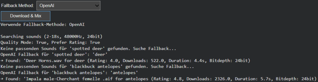
Building upon the intelligent fallback systems developed in Phase III, this week’s development addressed a more subtle yet critical challenge in audio generation: ensuring that retrieved sounds semantically match their visual counterparts. While the fallback system successfully handled missing sounds, I discovered that even when sounds were technically available, they didn’t always represent the intended objects accurately. This phase introduces a sophisticated description verification layer and flexible filtering system that transforms sound retrieval from a mechanical matching process to a semantically intelligent selection.

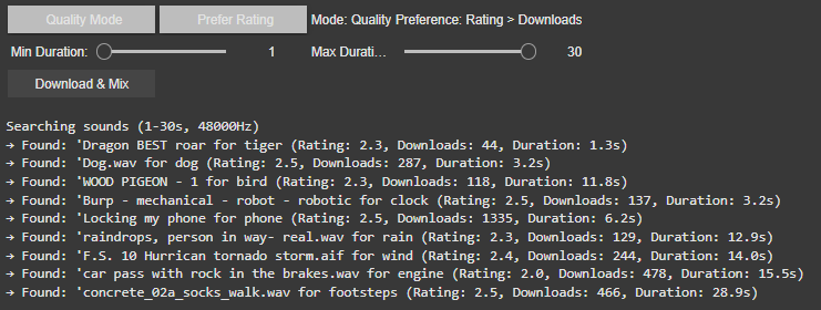
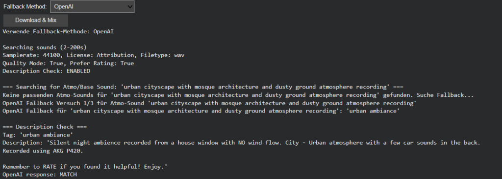
The newly implemented description verification system addresses this through OpenAI-powered semantic analysis. Each retrieved sound’s description is now evaluated against the original visual tag to determine if it represents the actual object or just references it contextually. This ensures that when Image Extender layers “car” sounds into a mix, they’re authentic engine recordings rather than musical tributes.

Intelligent Filter Architecture: Balancing Precision and Flexibility

Recognizing that overly restrictive filtering could eliminate viable sounds, we redesigned the filtering system with adaptive “any” options across all parameters. The Bit-Depth filter got removed because it resulted in search errors which is also mentioned in the documentation of the freesound.org api.

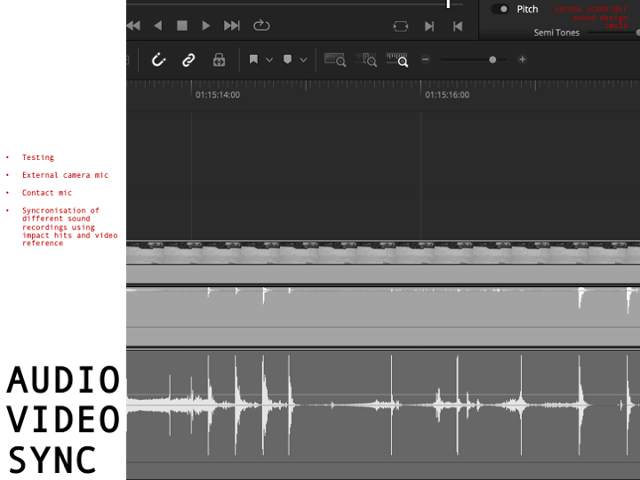
Scene-Aware Audio Composition: Atmo Sounds as Acoustic Foundation

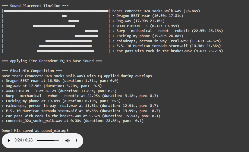
A significant architectural improvement involves intelligent base track selection. The system now distinguishes between foreground objects and background atmosphere:

  • Scene & Location Analysis: Object detection extracts environmental context (e.g., “forest atmo,” “urban street,” “beach waves”)
  • Atmo-First Composition: Background sounds are prioritized as the foundational layer
  • Stereo Preservation: Atmo/ambience sounds retain their stereo imaging for immersive soundscapes
  • Object Layering: Foreground sounds are positioned spatially based on visual detection coordinates

This creates mixes where environmental sounds form a coherent base while individual objects occupy their proper spatial positions, resulting in professionally layered audio compositions.

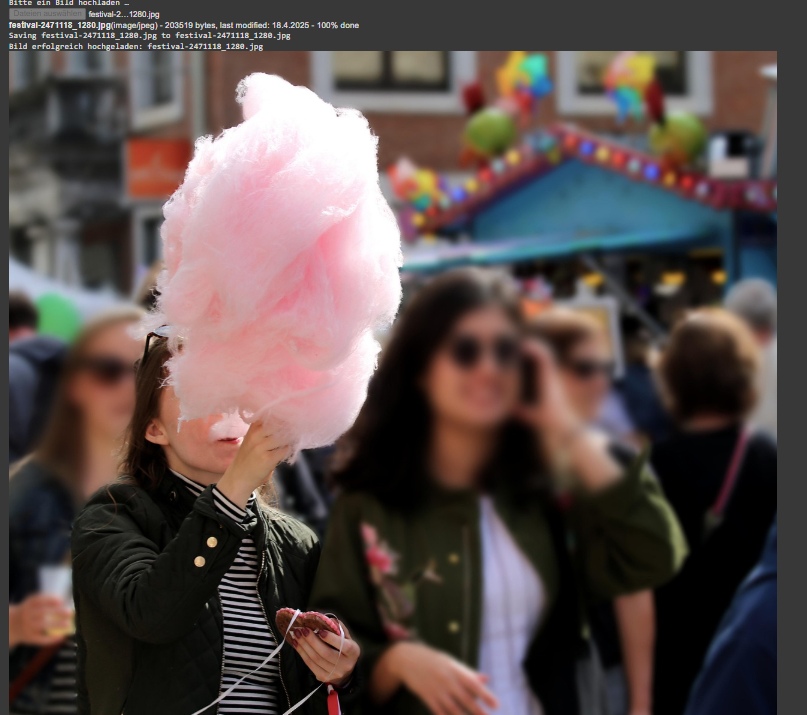
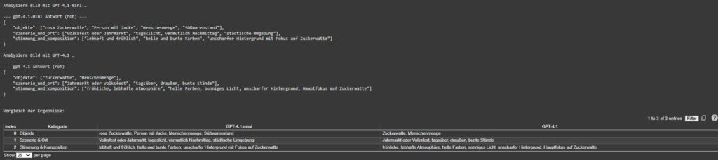
Dual-Mode Object Detection with Scene Understanding

OpenAI GPT-4.1 Vision: Provides comprehensive scene analysis including:

  • Object identification with spatial positioning
  • Environmental context extraction
  • Mood and atmosphere assessment
  • Structured semantic output for precise sound matching

MediaPipe EfficientDet: Offers lightweight, real-time object detection:

  • Fast local processing without API dependencies
  • Basic object recognition with positional data
  • Fallback when cloud services are unavailable

Wildcard-Enhanced Semantic Search: Beyond Exact Matching

Multi-Stage Fallback with Verification Limits

The fallback system evolved into a sophisticated multi-stage process:

  1. Atmo Sound Prioritization: Scene_and_location tags are searched first as base layer
  2. Object Search: query with user-configured filters
  3. Description Verification: AI-powered semantic validation of each result
  4. Quality Tiering: Progressive relaxation of rating and download thresholds
  5. Pagination Support: Multiple result pages when initial matches fail verification
  6. Controlled Fallback: Limited OpenAI tag regeneration with automatic timeout

This structured approach prevents infinite loops while maximizing the chances of finding appropriate sounds. The system now intelligently gives up after reasonable attempts, preventing computational waste while maintaining output quality.

Toward Contextually Intelligent Audio Generation

This week’s enhancements represent a significant leap from simple sound retrieval to contextually intelligent audio selection. The combination of semantic verification, adaptive filtering and scene-aware composition creates a system that doesn’t just find sounds, it finds the right sounds and arranges them intelligently.

Product III: Image Extender

Intelligent Sound Fallback Systems – Enhancing Audio Generation with AI-Powered Semantic Recovery

After refining Image Extender’s sound layering and spectral processing engine, this week’s development shifted focus to one of the system’s most practical yet creatively crucial challenges: ensuring that the generation process never fails silently. In previous iterations, when a detected visual object had no directly corresponding sound file in the Freesound database, the result was often an incomplete or muted soundscape. The goal of this phase was to build an intelligent fallback architecture—one capable of preserving meaning and continuity even in the absence of perfect data.

Closing the Gap Between Visual Recognition and Audio Availability

During testing, it became clear that visual recognition is often more detailed and specific than what current sound libraries can support. Object detection models might identify entities like “Golden Retriever,” “Ceramic Cup,” or “Lighthouse,” but audio datasets tend to contain more general or differently labeled entries. This mismatch created a semantic gap between what the system understands and what it can express acoustically.

The newly introduced fallback framework bridges this gap, allowing Image Extender to adapt gracefully. Instead of stopping when a sound is missing, the system now follows a set of intelligent recovery paths that preserve the intent and tone of the visual analysis while maintaining creative consistency. The result is a more resilient, contextually aware sonic generation process—one that doesn’t just survive missing data, but thrives within it.

Dual Strategy: Structured Hierarchies and AI-Powered Adaptation

Two complementary fallback strategies were introduced this week: one grounded in structured logic, and another driven by semantic intelligence.

The CSV-based fallback system builds on the ontology work from the previous phase. Using the tag_hierarchy.csv file, each sound tag is part of a parent–child chain, creating predictable fallback paths. For example, if “tiger” fails, the system ascends to “jungle,” and then “nature.” This rule-based approach guarantees reliability and zero additional computational cost, making it ideal for large-scale batch operations or offline workflows.

In contrast, the AI-powered semantic fallback uses GPT-based reasoning to dynamically generate alternative tags. When the CSV offers no viable route, the model proposes conceptually similar or thematically related categories. A specific bird species might lead to the broader concept of “bird sounds,” or an abstract object like “smartphone” could redirect to “digital notification” or “button click.” This layer of intelligence brings flexibility to unfamiliar or novel recognition results, extending the system’s creative reach beyond its predefined hierarchies.

User-Controlled Adaptation

Recognizing that different projects require different balances between cost, control, and creativity, the fallback mode is now user-configurable. Through a simple dropdown menu, users can switch between CSV Mode and AI Mode.

  • CSV Mode favors consistency, predictability, and cost-efficiency—perfect for common, well-defined categories.
  • AI Mode prioritizes adaptability and creative expansion, ideal for complex visual inputs or unique scenes.

This configurability not only empowers users but also represents a deeper design philosophy: that AI systems should be tools for choice, not fixed solutions.

Toward Adaptive and Resilient Multimodal Systems

This week’s progress marks a pivotal evolution from static, database-bound sound generation to a hybrid model that merges structured logic with adaptive intelligence. The dual fallback system doesn’t just fill gaps, it embodies the philosophy of resilient multimodal AI, where structure and adaptability coexist in balance.

The CSV hierarchy ensures reliability, grounding the system in defined categories, while the AI layer provides flexibility and creativity, ensuring the output remains expressive even when the data isn’t. Together, they form a powerful, future-proof foundation for Image Extender’s ongoing mission: transforming visual perception into sound not as a mechanical translation, but as a living, interpretive process.

Product I: Image Extender

OpenAI API Image Analyzer – Structured Vision Testing and Model Insights

Adaptive Visual Understanding Framework
In this development phase, the focus was placed on building a robust evaluation framework for OpenAI’s multimodal models (GPT-4.1 and GPT-4.1-mini). The primary goal: systematically testing image interpretation, object detection, and contextual scene recognition while maintaining controlled cost efficiency and analytical depth.

upload of image (image source: https://www.trumau.at/)
  1. Combined Request Architecture
    Unlike traditional multi-call pipelines, the new setup consolidates image and text interpretation into a single API request. This streamlined design prevents token overhead and ensures synchronized contextual understanding between categories. Each inference returns a structured Python dictionary containing three distinct analytical branches:
    • Objects – Recognizable entities such as animals, items, or people
    • Scene and Location Estimation – Environment, lighting, and potential geographic cues
    • Mood and Composition – Aesthetic interpretation, visual tone, and framing principles

For each uploaded image, the analyzer prints three distinct lists per modelside by side. This offers a straightforward way to assess interpretive differences without complex metrics. In practice, GPT-4.1 tends to deliver slightly more nuanced emotional and compositional insights, while GPT-4.1-mini prioritizes concise, high-confidence object recognition.

results of the image object analysis and model comparison

Through the unified format, post-processing can directly populate separate lists or database tables for subsequent benchmarking, minimizing parsing latency and data inconsistencies.

  1. Robust Output Parsing
    Because model responses occasionally include Markdown code blocks (e.g., python {…}), the parsing logic was redesigned with a multi-layered interpreter using regex sanitation and dual parsing strategies (AST > JSON > fallback). This guarantees that even irregularly formatted outputs are safely converted into structured datasets without manual intervention. The system thus sustains analytical integrity under diverse prompt conditions.
  2. Model Benchmarking: GPT-4.1-mini vs. GPT-4.1
    The benchmark test compared inference precision, descriptive richness, and token efficiency between the two models. While GPT-4.1 demonstrates deeper contextual inference and subtler mood detection, GPT-4.1-mini achieves near-equivalent recognition accuracy at approximately one-tenth of the cost per request. For large-scale experiments (e.g., datasets exceeding 10,000 images), GPT-4.1-mini provides the optimal balance between granularity and economic viability.
  3. Token Management and Budget Simulation
    A real-time token tracker revealed an average consumption of ~1,780 tokens per image request. Given GPT-4.1-mini’s rate of $0.003 / 1k tokens, a one-dollar operational budget supports roughly 187 full image analyses. This insight forms the baseline for scalable experimentation and budget-controlled automation workflows in cloud-based vision analytics.

The next development phase will integrate this OpenAI-driven visual analysis directly into the Image Extender environment. This integration marks the transition from isolated model testing toward a unified generative framework.

Playback and Visualization of x-IMU3 Sensor Data Using Python and Pure Data

Moving forward, in this section the documentation of the workflow used to playback recorded x-IMU3 motion sensor data and visualize it as a dynamic graph in Pure Data, is shown. The goal here was to analyze the movement of two specific flips along the X-axis. Therefore a few seconds of this rotation were recorded and then read through the python script, send to PureData and here printed in a visual graph. The confirmation of the accuracy was done through multiple validation layers.

First, data was captured using the x-IMU3 inertial measurement unit. During the recorded session, the sensor was physically maneuvered to do two flips along its X-axis. Then, this data was saved internally by the sensor into a binary format with the extension. ximu3. In order to later find this file again, it was named XIMUA_0005.ximu3 and was stored on an external drive.

Second step was to decode and transmit the recorded motion data. Therefore, I used a Python script named ximu2osc.py. This script was written to read both live and recorded data and transmit it via the Open Sound Control (OSC) protocol. This python script uses the official ximu3 Python library to do file decoding, and the python-osc library for sending OSC messages.

The python script was executed using the following command in the terminal:

Using this script the playback of the sensor recording get initialized by naming the .ximu3 file as input. Looking at the command, the -p argument sets the OSC port to 9000. The -H argument points out the destination IP address, which in this case is 127.0.0.1. The Python script, in the next step, reads and decodes the binary sensor data in real time. Next step, the formatted OSC messages gets send using a clearly defined path.

Focusing on the receiving end, a Pure Data (Pd) patch was created to receive and interpret the data. This patch was configured to listen on port 9000 and processes the incoming OSC messages with the [netreceive -u -b 9000] object. It is capable of receiving UDP packets in binary format. The output from netreceive was then connected into [oscparse] object. OSCPARSE is responsible for decoding incoming OSC messages into usable Pd lists.

[list trim] was introduced in the patch to remove any resisting selectors. As the next step, a set of [route] objects were implemented. There were placed to filter out the gyroscope data, specifically the values from the X, Y, and Z axes. In this process a hierarchical routing structure was used. The first one: [route intertial], followed by [route gyroscope] and finally [route xyz]. The final values were then unpacked using [unpack f f f] to split them into three float values (X, Y, Z). For this test, only the X-axis values were needed.

To have a visual representation of the X-axis values in real time, an array named array1 was created. It functions as a scrolling plot reading the incoming rotation data. This was executed by assigning each X value to a new index in the array [tabwrite array1]. A simple counter system was built using [metro] to write the position in the array. [+ 1], [mod 500]. The [metro] object gets triggered at a 500ms interval, which, in this case served as the sampling rate of the graph. This counter also loops over a fixed range of 500 steps. This is how the circular buffer was build. Now, each new value is being stored in a float object [f] and sent via [s x-index] to its matching [r x-index].

A screenshot of a computer

AI-generated content may be incorrect.

With using this setup, it is possible to visually plot the continuous stream of X-axis values into the array. The result is a dynamic visualization of the sensor’s movement over time. Looking at the playback of the recorded. ximu3 file, the two flips performed on the X-axis are strongly stown as spikes in the plotted graph. This provides a real representation of the motion of the flip along the X-axis. In addition, all values were also printed to the Pd console in order to verify and debugging purposes.

Next step, to ensure the accuracy of the visualization, I compared the received values in three different ways. First, I monitored the terminal output of the Python script. Here every OSC message that was being sent was printed out, including its path and its matching values. Secondly, I checked the values listed inside Pure Data. Here the numbers were compared with the one from the terminal. Thirdly, I opened the. ximu3 file in the official x-IMU3 GUI and therefore exported the data as a CSV file. Analyzing the resulting file Inertial.csv, the “Gyroscope X (deg/s)” column was detected and housing the same values then printed in the terminal, in Pure Data and visually on the graph. This lets me confirm, that the sensor data was transmitted consistently across all three layers: the original file, the terminal stream, and in the end, the Pd visualization.

In conclusion, this test showcasts a successful connection between recorded sensor movement and its visual representation using an OSC streaming data pipeline. A clearly structured, repeatable method was used to analyze a specific gestures or physical event, recorded by the sensor. Furthermore, the system is adaptive and can be easily adjusted to visualize different values. It also sets the ground stone for other possibilities in sound design and audio adjustment in the further process.

Using x-IMU3 Python API for Live USB Data

In addition to decoding files using the x-IMU3 GUI, this project also focuses on utilized the Python library provided by x-io Technologies. Here sensor data can be streamed directly from the device via an USB connection. After successfully installing the ximu3 package with pip3 install ximu3, the provided example scripts of the GitHub repository’s Examples/Python were being used. In particular the usb_connection.py. (https://github.com/xioTechnologies/x-IMU3-Software) In the next step, after installing the ximu3 Python package via pip3 install ximu3, the script usb_connection.py was located and run from the external SSD directory /Volumes/Extreme SSD/surfboard/usbConnection.

To execute the script, the following terminal command was used:
   python3 /Volumes/Extreme\ SSD/surfboard/usbConnection/usb_connection.py

The next step is successfully executed once the x-IMU3 is detected. Here the user is prompted whether to print data messages or not. After enabling this, the terminal now displays live sensor data. This data set includes quaternions, Euler angles, gyroscope, and accelerometer data. It is noticeable, that this method bypasses the GUI and provides a direct access to sensor streams. This step enables a more flexible integration and a more advanced data mapping setup.

The full Python architecture includes modular scripts like connection.py, usb_connection.py, and helpers.py. These are handling low-level serial communication and parsing. This additional access pathway expands the projects versatility and opens doors for a more experimental workflow (x-io Technologies, 2024).

  1.  OSC Data Interpretation in Pure Data

The received OSC data is interpreted using a custom Pure Data patch (imu3neuerversuch22.04..pd), which serves as a bridge between sensor data and visual representation of the data. This patch listens for incoming OSC messages via the [udpreceive] and [unpackOSC] objects, parsing them into sub-addresses like /imu3/euler, /imu3/acceleration, and /imu3/gyroscope.

Each of these OSC paths carries a list of float values, which are unpacked using [unpack f f f] objects. The resulting individual sensor dimensions (e.g., x, y, z) are then routed to various subpatches or modules. Inside these subpatches, the values are scaled and normalized to fit the intended modulation range. For example:

  • Euler angles are converted into degrees and used to modulate stereo panning or spatial delay.
  • Z-axis acceleration is used as a trigger threshold to initiate playback or synthesis grains.
  • Gyroscope rotation values modulate parameters like filter cutoff or reverb depth.

Additionally, [select] and [expr] objects are used to create logic conditions, such as identifying sudden peaks or transitions. This setup allows the system to treat physical gestures on the surfboard—like standing, carving, or jumping—as expressive control inputs for audio transformation.

The modular structure of the patch enables quick expansion. New OSC paths can be added, and new sound modules can be integrated without rewriting the core logic. By structuring the patch in this way, it remains both maintainable and flexible, supporting future extensions such as machine learning-based gesture classification or live improvisation scenarios.

This technical design reflects a broader trend in contemporary media art, where real-world data is used not just for visualization but as a means to dynamically sculpt immersive audio experiences (Puckette, 2007).

SOFTWARE AND DATA PIPELINE

    1.  Data Flow Overview

The data pipeline is structured in three different phases: acquisition, post-processing, and sonification. The first part, Acquisition includes independent capturing of audio (Zoom H4n, contact microphone), motion (x-IMU3), and video/audio (GoPro Hero 3). Then, in the next step, post-processing uses the x-IMU3 SDK to decode the recorded data. This data is then send via OSC to Pure Data and is there translated into its different parameters. 

The sonification and audio transformation are carried out also using Pure Data.

This architectural structure supports a secure workflow and easy synchronization in post.

  1. Motion Data Acquisition

Motion data was recorded onboard the x-IMU3 device. After each session, files were extracted using the x-IMU3 GUI and decoded into CSVs. These contain accelerometer, gyroscope, and orientation values with timestamps (x-io Technologies, 2024). Python scripts parsed the data and prepared OSC messages for transmission to Pure Data. The timing issue is faced with the help of synchronizing big movements in rotation or acceleration during the long recording all devices. (Wright et al., 2001).

The Audio recorded from the contact mic is a simple mono WAV file and is Pure Data and later Davinci Resolve for the audio video final cut. Looking at the recordings, the signal primarily consisted of strong impact sounds, board vibrations, water interactions and movements of the surfer. These recordings are used directly for the sound design of the movie. During the main part of the movie, when the surfer stands on the board, this audio will also be modulated using the motion data of the sensor reflecting on the gestures and board dynamics. (Puckette, 2007; Roads, 2001).

  1. Video and Sync Reference

Having all this different not in synchronized time recorded data files leaves a great question of exact synchronization. Therefore, a test was conducted which will be explained in more detail in the section: 10. SURF SKATE SIMULATION AND TEST RECORDINGS. The movement of surfing was simulated using a surf skateboard, on which a contact microphone was mounted on the bottom of the deck. In addition to the microphone also the motion sensor was placed next to the microphone. Now, having the image and the two sound sources (contact microphone and audio of the Sony camera) I could synchronize both recordings in post-production using Davinci Resolve. Here the main key findings were the importance of great labeling of the tracks and clear documentation of each recording. During the final recordings on the surfboard the GoPro Hero 3 will act as an important tool to synchronize all the different files in the end. Another audio output of the GoPro acts as an additional backup for a more stable synchronization workflow. Here test runs on the skateboard are essential to be able to manage all the files in post-production later.  (Watkinson, 2013).

The motion data recorded on the ximu3 sensor is replayed on the GUI of the sensor and can then send the data via OSC to Pure Data. Parameters such as pitch, roll, and vertical acceleration can then be mapped to different variables like grain density, stereo width, or filter cutoff frequency. (Puckette, 2007).

  1. Tools and Compatibility

All tools are selected based on compatibility and possibility to record under this special conditions. The toolchain includes:

  • x-IMU3 SDK and GUI (macOS) for sensor decoding
  • Python 3 for OSC streaming and data parsing
  • Pure Data for audio synthesis
  • DaVinci Resolve for editing and timeline alignment

This architecture functions as the basic groundwork of the project setup and can still be expanded using different software’s of python code to add more individualization during different steps of the process. (McPherson & Zappi, 2015).

  1.  Synchronization Strategy

Looking deeper into the Synchronization part of the project, challenges arrise. Because there is no global time setting for all devices, they have to run individually and then be synchronized in post-production. Here working with good documentation and clear labels of each track helps to get a good overview. Especially the data of the motion sensor will have a lot of information and needs to be time aligned with the audio. Synchronizing audio and video, however, is for sure a smaller challenge, because of the multiple different audio sources and the GoPro footage. A big impact or a strong turn of the board can then be mapped to the audio and video timeline. The advantage of one long recording of a 30 min surf session is for sure, that the possibility for such an event increase over time. Tests with the skateboard, external video and audio from the contact microphone were already successful.


On the image the setup in Davinci Resolved shows the synchronization of the contact microphone (pink) and the external audio of the Sony Alpha 7iii (green). Here the skateboard was hit against the floor in a rhythmical pattern, creating this noticeable spikes in audio on both devices. This rhythmical movement can also be seen on the XIMU3 sensor. 

Prototyping XI: Image Extender – Image sonification tool for immersive perception of sounds from images and new creation possibilities

Smart Sound Selection: Modes and Filters

1. Modes: Random vs. Best Result

  • Best Result Mode (Quality-Focused)
    The system prioritizes sounds with the highest ratings and download counts, ensuring professional-grade audio quality. It progressively relaxes standards (e.g., from 4.0+ to 2.5+ ratings) if no perfect match is found, guaranteeing a usable sound for every tag.
  • Random Mode (Diverse Selection)
    In this mode, the tool ignores quality filters, returning the first valid sound for each tag. This is ideal for quick experiments or when unpredictability is desired or to be sure to achieve different results.

2. Filters: Rating vs. Downloads

Users can further refine searches with two filter preferences:

  • Rating > Downloads
    Favors sounds with the highest user ratings, even if they have fewer downloads. This prioritizes subjective quality (e.g., clean recordings, well-edited clips).
    Example: A rare, pristine “tiger growl” with a 4.8/5 rating might be chosen over a popular but noisy alternative.
  • Downloads > Rating
    Prioritizes widely downloaded sounds, which often indicate reliability or broad appeal. This is useful for finding “standard” effects (e.g., a typical phone ring).
    Example: A generic “clock tick” with 10,000 downloads might be selected over a niche, high-rated vintage clock sound.

If there would be no matching sound for the rating or download approach the system gets to the fallback and uses the hierarchy table privided to change for example maple into tree.

Intelligent Frequency Management

The audio engine now implements Bark Scale Filtering, which represents a significant improvement over the previous FFT peaks approach. By dividing the frequency spectrum into 25 critical bands spanning 20Hz to 20kHz, the system now precisely mirrors human hearing sensitivity. This psychoacoustic alignment enables more natural spectral adjustments that maintain perceptual balance while processing audio content.

For dynamic equalization, the system features adaptive EQ Activation that intelligently engages only during actual sound clashes. For instance, when two sounds compete at 570Hz, the EQ applies a precise -4.7dB reduction exclusively during the overlapping period.

o preserve audio quality, the system employs Conservative Processing principles. Frequency band reductions are strictly limited to a maximum of -6dB, preventing artificial-sounding results. Additionally, the use of wide Q values (1.0) ensures that EQ adjustments maintain the natural timbral characteristics of each sound source while effectively resolving masking issues.

These core upgrades collectively transform Image Extender’s mixing capabilities, enabling professional-grade audio results while maintaining the system’s generative and adaptive nature. The improvements are particularly noticeable in complex soundscapes containing multiple overlapping elements with competing frequency content.

Visualization for a better overview

The newly implemented Timeline Visualization provides unprecedented insight into the mixing process through an intuitive graphical representation.

Experiment IV: Embodied Resonance – plot HRV metrics with python

Before we can compare a “healthy” and a “clinical” heart, we first need a small tool-chain that does three things automatically:

  1. detects each normal-to-normal (NN) beat in a raw ECG trace,
  2. converts those beats into the core HRV metrics (HR, SDNN, RMSSD, VLF, LF, HF, LF/HF) and
  3. plots every curve on an interactive dashboard so that trends can be inspected side-by-side.

Because the long-term goal is a live installation (eventually driving MIDI or other real-time mappings), the script is written from the start in a sliding-window style: at every step it re-computes each metric over a moving chunk of data.
Fast-changing variables such as heart-rate itself can use short windows and small hops; spectral indices need at least a five-minute span to remain physiologically trustworthy. Shortening that span may make the curves look “lively,” but it also distorts the underlying autonomic picture and breaks any attempt to compare one participant with another. The code therefore lets the user set an independent window length and step size for the time-domain group and for the frequency-domain group.
Let’s take a closer look at the code. If you want to see the full, visit: https://github.com/ninaeba/EmbodiedResonance

1. Imports and global parameters

import argparse
import sys
from pathlib import Path

import numpy as np
import pandas as pd
import plotly.graph_objs as go
import scipy.signal as sg
import neurokit2 as nk
  • argparse – give the script a tiny command-line interface so we can point it at any raw ECG CSV.
  • NumPy / pandas – basic numeric work and table handling.
  • scipy.signal – classic DSP tools (Butterworth filter, Lomb–Scargle).
  • neurokit2 – robust, well-tested R-peak detector.
  • plotly – interactive plotting inside a browser/Notebook; easy zooming for visual QA.

2. Tunable experiment-wide constants

FS_ECG   = 500              # ECG sample-rate (Hz)
BP_ECG   = (0.5, 40)        # band-pass corner frequencies

TIME_WIN, TIME_STEP = 60.0, 1.0   # sliding window for HR / SDNN / RMSSD
FREQ_WIN, FREQ_STEP = 300.0, 30.0   # sliding window for VLF / LF / HF
FGRID = np.arange(0.003, 0.401, 0.001)

BANDS = dict(VLF=(.003, .04), LF=(.04, .15), HF=(.15, .40))
  • Butterworth 0.5–40 Hz is a widely used cardiology band-pass that suppresses baseline wander and high-frequency EMG, yet leaves the QRS complex untouched.
  • 60s time-domain window strikes a balance: long enough to tame noise, short enough for semi-real-time trend tracking.
  • 300s spectral window is deliberately longer; the literature shows that the lower bands (especially VLF) are unreliable below ~5 min.
  • FGRID – dense frequency grid (1 mHz spacing) for a smoother Lomb curve.

3. ECG helper class – load, (optionally) filter, detect R-peaks

class ECG:
def __init__(self, fs=FS_ECG, bp=BP_ECG, use_filter=True):
...
def load(self, fname: Path) -> np.ndarray:
...
def filt(self, sig):
...
def r_peaks(self, sig_f):
...
  1. load – reads the CSV into a flat float vector and sanity-checks that we have >10 s of data.
  2. filt – if the --nofilt flag is absent, applies a 4-th-order zero-phase Butterworth band-pass (via filtfilt) so that the baseline drift of slow breathing (or cable motion) does not trick the peak detector.
  3. r_peaks – delegates the hard work to neurokit2.ecg_process, which combines Pan-Tompkins-style amplitude heuristics with adaptive thresholds; returns index positions and their timing in seconds.

4. HRV class – sliding-window metric engine

class HRV:
...
def time_metrics(rr):
...
def lomb_bandpowers(self, rr, t_rr):
...
def time_series(self, r_t):
...
def freq_series(self, r_t):
...
def compute(self, r_t):
...
  • time_metrics converts every RR sub-series into three classic metrics
    HR (beats/min), SDNN (overall beat-to-beat spread, ms), RMSSD (short-term jitter, ms).
  • Why Lomb–Scargle instead of Welch?
    The RR intervals are unevenly spaced by definition.
    • Welch needs evenly sampled tachograms or heavy interpolation → can distort the spectrum.
    • Lomb operates directly on irregular timestamps, preserving low-frequency content even if breathing or motion momentarily speeds up/slows down the heart.
  • lomb_bandpowers:
    1. Runs scipy.signal.lombscargle on de-trended RR values.
    2. Integrates power inside canonical VLF / LF / HF bands.
    3. Computes LF/HF ratio, but guards against division by tiny HF values.
  • time_series / freq_series slide a window (120 s or 300 s) across the experiment, jump every 30 s, calculate metrics, and store the mid-window timestamp for plotting.
  • compute finally stitches time-domain and frequency-domain rows onto a 1-second master grid so that all curves overlay cleanly.

5. Tiny colour dictionary

COLORS = dict(HR='#d62728', SDNN='#2ca02c', RMSSD='#ff7f0e',
VLF='#1f77b4', LF='#17becf', HF='#bcbd22', LF_HF='#7f7f7f')

Just cosmetic – keeps HR red, SDNN green, etc., across all subjects so eyeballing becomes effortless.


6. plot() – interactive dashboard

def plot(ecg_f, hrv_df, fs=FS_ECG, title="HRV (Lomb)"):
...
  • Left y-axis = filtered ECG trace for QC (do peaks line up?).
  • Right y-axis = every HRV curve.
  • Built-in range-slider lets you scrub the 24-minute protocol quickly.
  • Hover shows exact numeric values (handy when you are screening anomalies).
  • different backgrounds for phases

7. CLI wrapper

if __name__ == '__main__':
main()

Inside main() we parse the file name and the --nofilt flag, run the whole pipeline, save the HRV table as a CSV sibling (same stem, suffix .hrv_lomb.csv) and open the Plotly window.


The four summary plots included below are therefore not an end-point but a launch-pad: they give us a quick visual fingerprint of each participant’s autonomic response, and will serve as the reference material for deeper statistical comparison, pattern-searching, and—ultimately—the data-to-sound (or other real-time) mappings we plan to build next.

Prototyping X: Image Extender – Image sonification tool for immersive perception of sounds from images and new creation possibilities

Researching Automated Mixing Strategies for Clarity and Real-Time Composition

As the Image Extender project continues to evolve from a tagging-to-sound pipeline into a dynamic, spatially aware audio compositing system, this phase focused on surveying and evaluating recent methods in automated sound mixing. My aim was to understand how existing research handles spectral masking, spatial distribution, and frequency-aware filtering—especially in scenarios where multiple unrelated sounds are combined without a human in the loop.

This blog post synthesizes findings from several key research papers and explores how their techniques may apply to our use case: a generative soundscape engine driven by object detection and Freesound API integration. The next development phase will evaluate which of these methods can be realistically adapted into the Python-based architecture.

Adaptive Filtering Through Time–Frequency Masking Detection

A compelling solution to masking was presented by Zhao and Pérez-Cota (2024), who proposed a method for adaptive equalization driven by masking analysis in both time and frequency. By calculating short-time Fourier transforms (STFT) for each track, their system identifies where overlap occurs and evaluates the masking directionality—determining whether a sound acts as a masker or a maskee over time.

These interactions are quantified into masking matrices that inform the design of parametric filters, tuned to reduce only the problematic frequency bands, while preserving the natural timbre and dynamics of the source sounds. The end result is a frequency-aware mixing approach that adapts to real masking events rather than applying static or arbitrary filtering.

Why this matters for Image Extender:
Generated mixes often feature overlapping midrange content (e.g., engine hums, rustling leaves, footsteps). By applying this masking-aware logic, the system can avoid blunt frequency cuts and instead respond intelligently to real-time spectral conflicts.

Implementation possibilities:

  • STFTs: librosa.stft
  • Masking matrices: pairwise multiplication and normalization (NumPy)
  • EQ curves: second-order IIR filters via scipy.signal.iirfilter

“This information is then systematically used to design and apply filters… improving the clarity of the mix.”
— Zhao and Pérez-Cota (2024)

Iterative Mixing Optimization Using Psychoacoustic Metrics

Another strong candidate emerged from Liu et al. (2024), who proposed an automatic mixing system based on iterative masking minimization. Their framework evaluates masking using a perceptual model derived from PEAQ (ITU-R BS.1387) and adjusts mixing parameters—equalization, dynamic range compression, and gain—through iterative optimization.

The system’s strength lies in its objective function: it not only minimizes total masking but also seeks to balance masking contributions across tracks, ensuring that no source is disproportionately buried. The optimization process runs until a minimum is reached, using a harmony search algorithm that continuously tunes each effect’s parameters for improved spectral separation.

Why this matters for Image Extender:
This kind of global optimization is well-suited for multi-object scenes, where several detected elements contribute sounds. It supports a wide range of source content and adapts mixing decisions to preserve intelligibility across diverse sonic elements.

Implementation path:

  • Masking metrics: critical band energy modeling on the Bark scale
  • Optimization: scipy.optimize.differential_evolution or other derivative-free methods
  • EQ and dynamics: Python wrappers (pydub, sox, or raw filter design via scipy.signal)

“Different audio effects… are applied via an iterative Harmony searching algorithm that aims to minimize the masking.”
— Liu et al. (2024)

Comparative Analysis

MethodCore ApproachIntegration PotentialImplementation Effort
Time–Frequency Masking (Zhao)Analyze masking via STFT; apply targeted EQHigh — per-event conflict resolutionMedium
Iterative Optimization (Liu)Minimize masking metric via parametric searchHigh — global mix clarityHigh

Both methods offer significant value. Zhao’s system is elegant in its directness—its per-pair analysis supports fine-grained filtering on demand, suitable for real-time or batch processes. Liu’s framework, while computationally heavier, offers a holistic solution that balances all tracks simultaneously, and may serve as a backend “refinement pass” after initial sound placement.

Looking Ahead

This research phase provided the theoretical and technical groundwork for the next evolution of Image Extender’s audio engine. The next development milestone will explore hybrid strategies that combine these insights:

  • Implementing a masking matrix engine to detect conflicts dynamically
  • Building filter generation pipelines based on frequency overlap intensity
  • Testing iterative mix refinement using masking as an objective metric
  • Measuring the perceived clarity improvements across varied image-driven scenes

References

Zhao, Wenhan, and Fernando Pérez-Cota. “Adaptive Filtering for Multi-Track Audio Based on Time–Frequency Masking Detection.” Signals 5, no. 4 (2024): 633–641. https://doi.org/10.3390/signals5040035:contentReference[oaicite:2]{index=2}

Liu, Xiaojing, Angeliki Mourgela, Hongwei Ai, and Joshua D. Reiss. “An Automatic Mixing Speech Enhancement System for Multi-Track Audio.” arXiv preprint arXiv:2404.17821 (2024). https://arxiv.org/abs/2404.17821:contentReference[oaicite:3]{index=3}

Prototyping VIII: Image Extender – Image sonification tool for immersive perception of sounds from images and new creation possibilities

Sound-Image Matching via Semantic Tag Comparison

Continuing development on the Image Extender project, I’ve been exploring how to improve the connection between recognized visual elements and the sounds selected to represent them. A key question in this phase has been: How do we determine if a sound actually fits an image, not just technically but meaningfully?

Testing the Possibilities

I initially looked into using large language models to evaluate the fit between sound descriptions and the visual content of an image. Various API-based models showed potential in theory, particularly for generating a numerical score representing how well a sound matched the image content. However, many of these options required paid access or more complex setup than suited this early prototyping phase. I also explored frameworks like LangChain to help with integration, but these too proved a bit unstable for the lightweight, quick feedback loops I was aiming for.

A More Practical Approach: Semantic Comparison

To keep things moving forward, I’ve shifted toward a simpler method using semantic comparison between the image content and the sound description. In this system, the objects recognized in an image are merged into a combined tag string, which is then compared against the sound’s description using a classifier that evaluates their semantic relatedness.

Rather than returning a simple yes or no, this method provides a score that reflects how well the description aligns with the image’s content. If the score falls below a certain threshold, the sound is skipped — keeping the results focused and relevant without needing manual curation.

Why It Works (for Now)

This tag-based comparison system is easy to implement, doesn’t rely on external APIs, and integrates cleanly into the current audio selection pipeline. It allows for quick iteration, which is key during the early design and testing stages. While it doesn’t offer the nuanced understanding of a full-scale LLM, it provides a surprisingly effective filter to catch mismatches between sounds and images.

In the future, I may revisit the idea of using larger models once a more stable or affordable setup is in place. But for this phase, the focus is on building a clear and functional base — and semantic tag matching gives just enough structure to support that.