After completing the hardware setup, the next step was to verify whether the system was capable of producing usable physiological signals. For this purpose, a minimal Arduino sketch was written to read raw analog values from the ECG and GSR sensors and stream them via the serial interface. The goal at this stage was not data recording or analysis, but a basic functional test of the signal paths. The code continuously reads the ECG signal from analog input A1 and the GSR signal from analog input A2, printing both values as comma-separated numbers to the Serial Monitor. A short delay was introduced to limit the sampling rate and ensure stable serial transmission.
const int ecgPin = A1;
const int gsrPin = A2;
void setup() {
Serial.begin(115200);
}
void loop() {
int ecgValue = analogRead(ecgPin);
int gsrValue = analogRead(gsrPin);
// print CSV row: ecg,gsr
Serial.print(ecgValue);
Serial.print(“,”);
Serial.println(gsrValue);
delay(5);
}
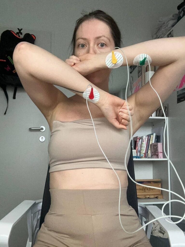
Once the code was running, the next critical step was the physical placement of the ECG electrodes. This proved to be one of the most challenging parts of the initial testing phase. Online sources provide a wide range of DIY electrode placement schemes, many of which are inconsistent or oversimplified. In particular, a previously referenced HRV-related Arduino project suggested placing electrodes on the arms. This configuration was tested first, but the resulting signal made it difficult to identify clear R-peaks in the serial plotter, which are essential for ECG interpretation and HRV analysis.
Example of ECG electrode placement as proposed in the “Arduino and HRV Analysis” project and author’s implementation. https://emersonkeenan.net/arduino-hrv/
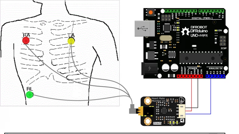
The official documentation of the ECG sensor instead recommended chest-based electrode placement. However, this approach also required careful positioning to achieve a clean signal.
ECG electrode placement on the chest as recommended in the official sensor documentation.
The most reliable guidance was found in a tutorial video presented by a medical professional, which explained proper ECG electrode placement in practical terms. The key insight was that electrodes should not be placed directly on bone. Instead, they must be positioned on soft tissue—below the shoulder and above the rib cage.
The ECG cables were clearly labeled by the manufacturer:
L (left) electrode placed on the left side of the chest
R (right) electrode placed symmetrically on the right side
F (foot/reference) electrode placed on the lower left abdomen, below the rib cage
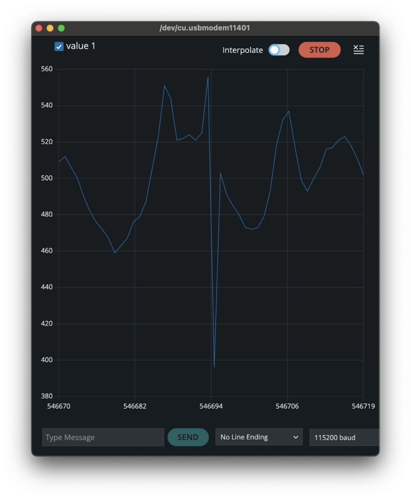
Additionally, skin preparation proved to be essential. Degreasing the skin before attaching the electrodes significantly improved signal quality. After applying these corrections and restarting the Arduino sketch, distinct ECG peaks became clearly visible in the serial output.
Raw ECG signal displayed in the Serial Plotter, showing clearly identifiable R-peaks during initial signal testing.
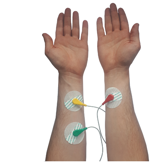
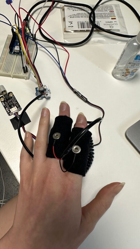
In contrast, the GSR sensor required far less preparation. It was simply attached to the fingers, and a signal was immediately observable. However, even during these initial tests it became evident that the GSR signal was highly noisy and would require filtering and post-processing in later stages of the project.
GSR sensor placement on the fingers during data acquisition.
Several practical limitations of the Arduino IDE became apparent during this testing phase. One major drawback was the inability to adjust the grid or scaling in the Serial Plotter, which made live signal inspection inconvenient. Furthermore, the current version of the Arduino IDE no longer allows direct export of serial data to CSV format from the monitor. This limitation necessitated additional tooling and custom scripts in later stages to enable proper data logging and analysis.
After converting heart-rate data into drums and HRV energy into melodic tracks, I needed a tiny helper that outputs nothing but automation. The idea was to pull every physiologic stream—HR, SDNN, RMSSD, VLF, LF, HF plus the LF / HF ratio—and stamp each one into its own MIDI track as CC-1 so that in the DAW every signal can be mapped to a knob, filter or layer-blend. The script must first look at all CSV files in a session, find the global minimum and maximum for every column, and apply those bounds consistently. Timing stays on the same 75 BPM / 0.1 s grid we used for the drums and notes, making one CSV row equal one 1⁄32-note. With that in mind, the core design is just constants, a value-to-CC rescaler, a loop that writes control changes, and a batch driver that walks the folder.
# ─── Default Configuration ───────────────────────────────────────────
DEF_BPM       = 75             # Default tempo
CSV_GRID      = 0.1            # Time between CSV samples (s) ≙ 1/32-note @75 BPM
SIGNATURE     = "8/8"          # Eight-cell bar; enough for pure CC data
CC_NUMBER     = 1              # We store everything on Mod Wheel
CC_TRACKS     = ["HR", "SDNN", "RMSSD", "VLF", "LF", "HF", "LF_HF"]
BEAT_PER_GRID = 1 / 32         # Grid resolution in beats
The first helper, map_to_cc, squeezes any value into the 0-127 range. It is the only place where scaling happens, so if you ever need logarithmic behaviour you change one line here and every track follows.
generate_cc_tracks loads a single CSV, back-fills gaps, creates one PrettyMIDI container and pins the bar length with a time-signature event. Then it iterates over CC_TRACKS; if the column exists it opens a fresh instrument named after the signal and sprinkles CC messages along the grid. Beat-to-second conversion is the same one-liner used elsewhere in the project.
for name in CC_TRACKS:
if name not in df.columns:
continue
vals = df[name].to_numpy()
vmin, vmax = minmax[name]
inst = pm.Instrument(program=0, is_drum=False, name=f"{name}_CC1")

for i in range(len(vals) - 1):
    beat = i * BEAT_PER_GRID * 4          # 1/32-note → quarter-note space
    t    = beat * 60.0 / bpm
    cc_val = map_to_cc(vals[i], vmin, vmax)
    inst.control_changes.append(
        pm.ControlChange(number=CC_NUMBER, value=cc_val, time=t)
    )

midi.instruments.append(inst)
The wrapper main is pure housekeeping: parse CLI flags, list every *.csv, compute global min-max per signal, and then hand each file to generate_cc_tracks. Consistent scaling is guaranteed because min-max is frozen before any writing starts.
minmax: dict[str, tuple[float, float]] = {}
for name in CC_TRACKS:
vals = []
for f in csv_files:
df = pd.read_csv(f, usecols=lambda c: c.upper() == name)
if name in df.columns:
vals.append(df[name].to_numpy())
if vals:
all_vals = np.concatenate(vals)
minmax[name] = (np.nanmin(all_vals), np.nanmax(all_vals))
Each CSV turns into *_cc_tracks.mid containing seven tracks—HR, SDNN, RMSSD, VLF, LF, HF, LF_HF—each packed with CC-1 data at 1⁄32-note resolution. Drop the file into Ableton, assign a synth or effect per track, map the Mod Wheel to whatever parameter makes sense, and the physiology animates the mix in real time.
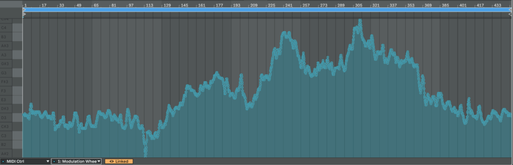
As a result, we get CC automation that we can easily map to something else or just copy automation somewhere else:
Here is an example of HR from patient 115 mapped from 0 to 127 in CC:
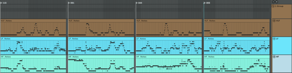
The next step after the drum generator is a harmonic layer built from frequency-domain HRV metrics. The script should do exactly what the drum code did for HR: scan all source files, find the global minima and maxima of every band, then map those values to pitches. Very-low-frequency (VLF) energy lives in the first octave, low-frequency (LF) in the second, high-frequency (HF) in the third. Each band is written to its own MIDI track so a different instrument can be assigned later, and every track also carries two automation curves: one CC lane for the band’s amplitude and one for the LF ⁄ HF ratio. In the synth that ratio will cross-fade between a sine and a saw: a large LF ⁄ HF—often a stress marker—makes the tone brighter and scratchier.
Instead of all twelve semitones, the script confines itself to the seven notes of C major or C minor. The mode flips in real time: if LF ⁄ HF drops below two the scale is major, above two it turns minor. Timing is flexible: each band can have its own step length and note duration so VLF moves more slowly than HF.
Below is a concise walk-through of ecg_to_notes.py. Key fragments of the code are shown inline for clarity. If you want to see the full, visit: https://github.com/ninaeba/EmbodiedResonance
# ----- core tempo & bar settings -----
DEF_BPM   = 75      # fixed song tempo
CSV_GRID  = 0.1     # raw data step in seconds
SIGNATURE = "8/8"   # eight cells per bar (fits VLF rhythms)
The script assigns a dedicated time grid, rhythmic value, and starting octave to each band. Those values are grouped in three parallel constants so you can retune the behaviour by editing one block.
Major and minor material is pre-baked as two simple interval lists. A helper translates any normalised value into a scale degree, then into an absolute MIDI pitch; another helper turns the same value into a velocity between 80 and 120 so you can hear amplitude without a compressor.
signals_to_midi opens one CSV, grabs the four relevant columns, and sets up three PrettyMIDI instruments—one per band. Inside a single loop the three arrays are processed identically, differing only in timing and octave. At each step the script decides whether we are in C major or C minor, converts the current value to a note and velocity, and appends the note to the respective instrument.
Every note time-stamp is paired with two controller messages: the first transmits the band amplitude, the second the LF / HF stress proxy. Both are normalised to the full 0-127 range so they can drive filters, wavetable morphs, or anything else in the synth.
The main wrapper gathers all CSVs in the chosen folder, computes global min–max values so every file shares the same mapping, and calls signals_to_midi on each source. Output files are named *_signals_notes.mid, each holding three melodic tracks plus two CC lanes per track. Together with the drum generator this completes the biometric groove: pulse drives rhythm, spectral power drives harmony, and continuous controllers keep the sound evolving.
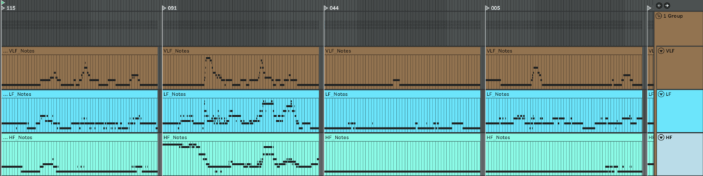
Here is what we get if we make one mappinf for all patients
An here is example of MIDI files we get if we make individual mapping for each patient separetly
To generate heart-rate–driven drums I set out to write a script that builds a drum pattern whose density depends on HR intensity. I fixed the tempo at 75 BPM because the math is convenient: 0.1 s of data ≈ one 1/32-note at 75 BPM. I pictured a bar with 16 cells and designed a map that decides which cell gets filled next; the higher the HR, the more cells are activated. Before rendering, a helper scans the global HR minimum and maximum and slices that span into 16 equal zones (an 8-zone fallback is available) so the percussion always scales correctly. For extra flexibility, the script also writes SDNN and RMSSD into the MIDI file as two separate CC automation lanes. In Ableton, I can map those controllers to any parameter, making it easy to experiment with the track’s sonic texture.
This script converts raw heart-rate data into a drum track. Every 0.1-second CSV sample lines up with a 1⁄32-note at the fixed tempo of 75 BPM, so medical time falls neatly onto a musical grid. The pulse controls how many cells inside each 16-step bar are filled, while SDNN and RMSSD are embedded as two CC lanes for later sound-design tricks.
Default configuration (all constants live in one block)
 STEP_BEAT = 1 / 32  # grid resolution in beats
 NOTE_LENGTH = 1 / 32  # each hit lasts a 32nd-note
 DEF_BPM = 75    # master tempo
 CSV_GRID = 0.1   # CSV step in seconds
 SEC_PER_CELL = 0.1   # duration of one pattern cell
 SIGNATURE = "16/16" # one bar = 16 cells
 CC_SDNN = 11    # long-term HRV
 CC_RMSSD = 1    # short-term HRV
The spatial order of hits is defined by a map that spreads layers across the bar, so extra drums feel balanced instead of bunching at the start
generate_rules slices the global HR span into sixteen equal zones and binds each zone to one cell-and-note pair; the last rule catches any pulse above the top threshold
 def generate_rules(hr_min, hr_max, cells):
  thresholds = np.linspace(hr_min, hr_max, cells + 1)[1:]
  rules = [(thr, CELL_MAP[i], 36 + i) for i, thr in enumerate(thresholds)]
  rules[-1] = (np.inf, rules[-1][1], rules[-1][2])
  return rules
Inside csv_to_midi the script first writes two continuous-controller streams—one for SDNN, one for RMSSD—normalised to 0-127 at every grid tick
 sdnn_norm = clip((sdnn − min) / (range), 0, 1)
 rmssd_norm = clip((rmssd − min) / (range), 0, 1)
 add CC 11 with value round(sdnn_norm × 127) at time t
 add CC 1 with value round(rmssd_norm × 127) at time t
A cumulative-pattern list is built so rhythmic density rises without ever muting earlier layers
 CUM_PATTERNS = []
 acc = []
 for (thr, cell, note) in rules:
  acc.append((cell, note)) # keep previous hits
  CUM_PATTERNS.append(list(acc)) # zone n holds n+1 hits
During rendering each bar/cell slot is visited, the current HR is interpolated onto that exact moment, its zone is looked up, velocity is set to the rounded pulse value, and only the cells active in that zone fire
 hr = interp(t_sample, times, hr_vals)
 zone = first i where hr ≤ rules[i].threshold
 vel = int(round(hr))
for (z_cell, note) in CUM_PATTERNS[zone]: if z_cell ≠ cell: continue beat = (bar × cells + cell) × STEP_BEAT × 4 t0 = beat × 60 / bpm write Note(pitch=note, velocity=vel, start=t0, end=t0 + NOTE_LENGTH in seconds)
Before any writing starts the entry-point scans the whole folder to gather global minima and maxima for HR, SDNN and RMSSD, guaranteeing identical zone limits and CC scaling across every file in the batch
 hr_min, hr_max = min/max of all HR values
 sdnn_min, sdnn_max = min/max of all SDNN values
 rmssd_min, rmssd_max = min/max of all RMSSD values
 rules = generate_rules(hr_min, hr_max, cells)
Each CSV becomes a _drums.mid file that contains a single drum-kit track whose note density follows heart-rate zones and whose CC 11 and CC 1 envelopes mirror long- and short-term variability—ready to animate filters, reverbs or whatever you map them to in the DAW.
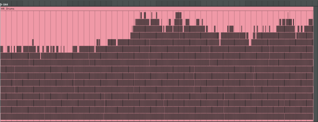
Here are examples of generated MIDI files with drums. On the left side, there are drums made with individual mapping for every patient separately, and on the right side, mapping is one for all patients. We can see they resemble our HR graphs.
Below are the four participants whose heart-rate-variability traces we have explored. We deliberately chose them because they sit at clearly different points on the “health–illness” spectrum and therefore give us a compact but vivid physiological palette.
Subject 119 is our practical baseline. No cardiac findings, no anxiety-or-depression scores, no PTSD, no “Type-D” personality pattern. Anything we hear or see in this person’s HRV should approximate the dynamics of an uncomplicated, resilient autonomic system.
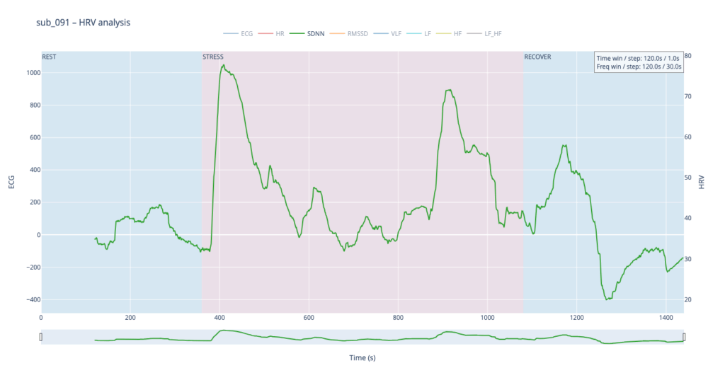
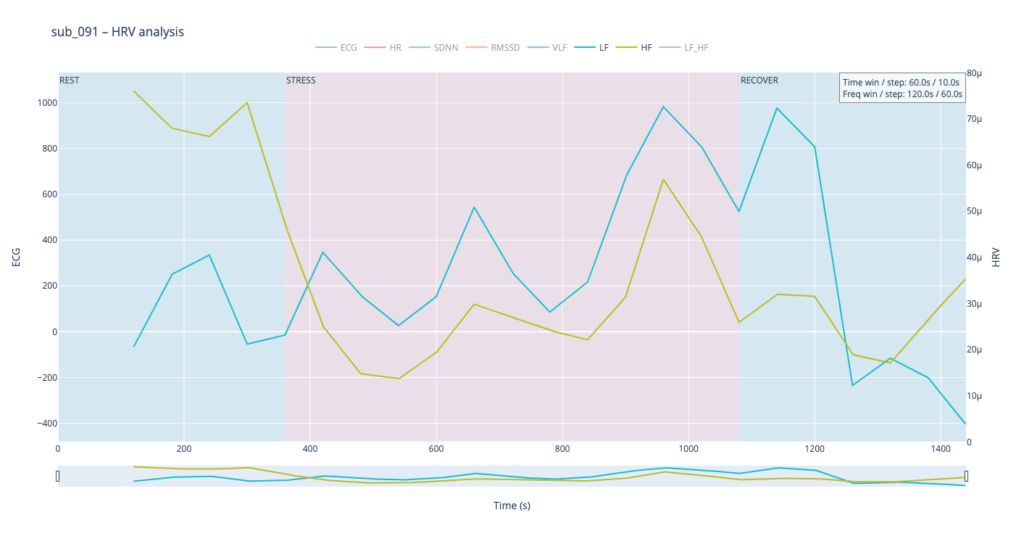
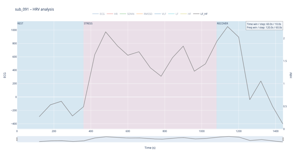
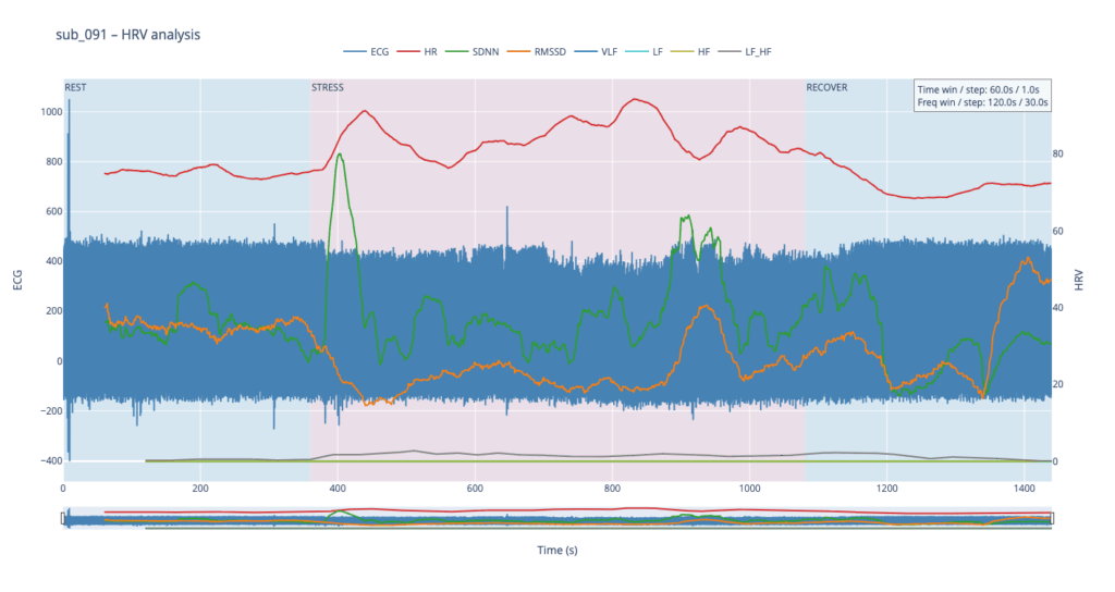
Subject 091 represents a “mind-only” disturbance. The heart itself is structurally sound, but the person carries the so-called Type-D trait (high negative affect, high social inhibition). This makes the autonomic system more reactive to worry or rumination even when the coronary vessels are normal.
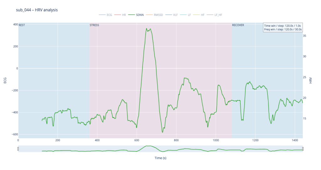
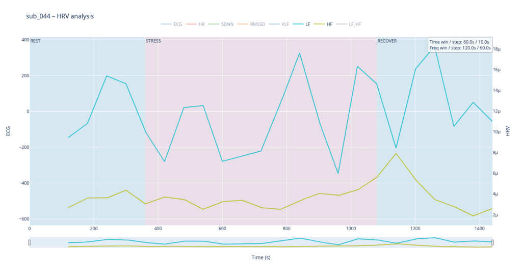
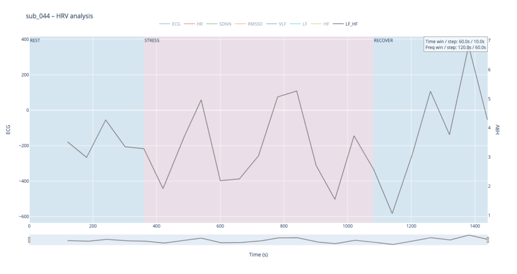
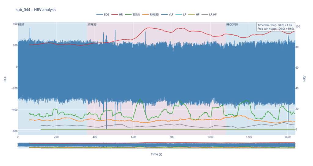
Subject 044 adds psychological trauma on top of mild, non-obstructive angina. Clinically this participant scores high on anxiety and meets full PTSD criteria. We therefore expect brisk sympathetic surges, slower vagal recovery and more noise in the LF/HF ratio—an autonomic pattern often seen in hyper-arousal states.
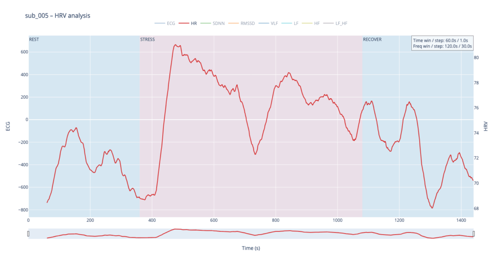
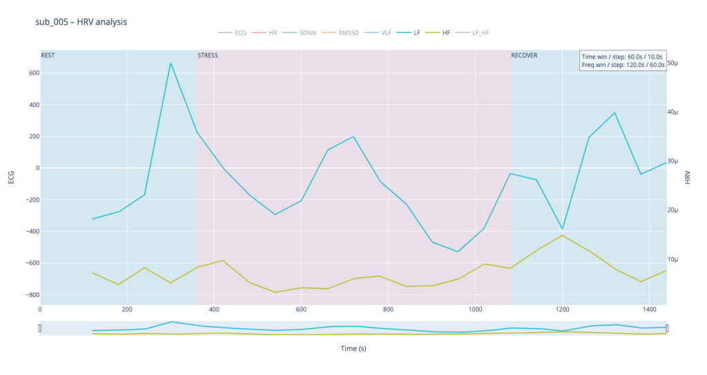
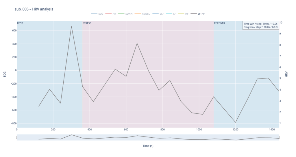
Subject 005 is the most medically burdened case: non-obstructive angina, endothelial dysfunction, stress-induced ischaemia, plus anxiety, depression, Type-D personality and PTSD. In short, both the mechanical pump and the emotional “software” are under strain, so variability measures are likely compressed and heart-rate plateaus may appear where a healthy person would fluctuate.
Using these four contrasting bodies as our “voices” lets us investigate how the same 6-min rest → 12-min exercise → 6-min recovery protocol is translated into four distinct autonomic narratives—information we will later map into equally distinct sonic textures.
HR
In general, each cardiovascular system answers physical load differently, depending on the baseline autonomic tone, fitness, psychological state, and comorbidities.
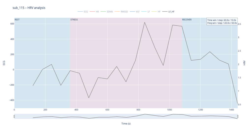
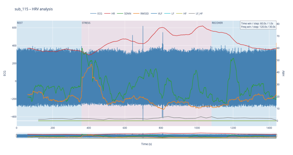
sub 115 – “healthy” The heart “ramps up” slowly. Pulse climbs in stair-like steps with brief dips between peaks—the body is constantly trying to regain homeostasis. After the exercise HR quickly falls almost to baseline. This is typical of a well-trained, adaptive cardiovascular system with a large functional reserve.
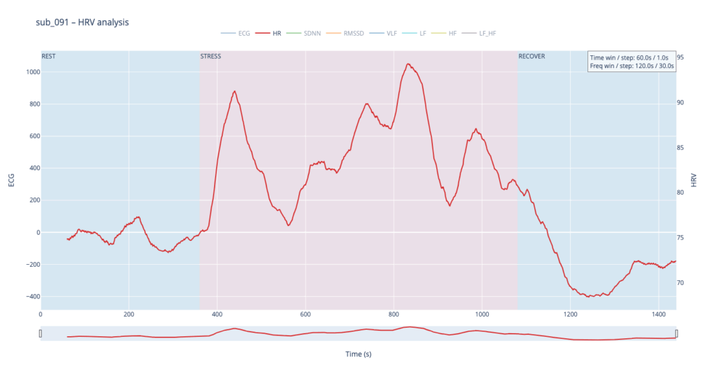
sub 091 – “mental / Type D” Resting HR is slightly above normal, yet overt anxiety is absent. The response is inertial: about a minute after load starts HR jumps from 75 → 91 bpm, then plummets to 76, followed by alternating short rises and falls. When the exercise stops, HR drops to 68 (below the initial value) and only then drifts back to ~75. Such a “swing” may reflect conflicting sympathetic vs. parasympathetic signals: outward calm while inner tension builds and discharges in bursts.
sub 044 – “PTSD” Even before load the heart is already in “fight-or-flight” mode (~83 bpm). The onset of exercise changes little, but at the third minute HR spikes to 98. It then declines stepwise yet remains high (89–97) even during recovery. The absence of a deep post-exercise dip shows that the parasympathetic “brake” hardly engages— the body struggles to shift into a resting state.
sub 005 – “sick / multiple pathologies” Baseline HR is 68. At the start of exercise it leaps to 80, after which it very slowly, step-by-step, drifts back toward normal and stays there until the end of the trial. The pattern resembles sub 044 but with lower background stress and slightly better recovery.
In healthy subjects the heart rate rises smoothly in step-like waves during effort and quickly settles back to baseline once the task stops, reflecting a well-balanced push-and-pull between sympathetic “accelerator” activity and parasympathetic (vagal) “brakes.” In patients with cardiac disease, PTSD or Type-D traits the resting rate is already elevated, the response to stress is sharper or more erratic, and the return to baseline is sluggish, showing a system locked in chronic “fight-or-flight” with weaker vagal damping.
Sound-design mapping:
Based on HR, I want to create drum patterns, where the lowest HR generates only kick, and then if HR rises, we can add more percusive elements.
SDNN
SDNN tracks how much the RR-intervals expand and shrink over time.
When the value climbs, the spacing between beats becomes more irregular—your heart is “dancing” around the mean to satisfy moment-to-moment demands.
When the value sinks, the intervals line up almost like a metronome—either the organism is in very deep rest or the rhythm is held in a tight sympathetic “clamp” and cannot flex.
Usually this parameter is calculated for 24 hours, but since we dont have such luxury, we stick to 2min time window
Looking at all four traces, the healthy control shows the widest SDNN swing and more frequent surges during the load phase. This wide dynamic range tells us the cardiac pacemaker is quick to loosen and tighten the rhythm, i.e. it adapts smoothly to the body’s changing needs. By contrast, the clinical subjects operate in a narrower corridor: their SDNN rarely strays far from baseline, signalling that the heart either remains compressed by chronic sympathetic tone or cannot recruit enough parasympathetic “slack” to respond fully.
For the sound-mapping layer, I’d like to add a short delay on the Drums track and control athe mount of feedback and reverb of echoes.
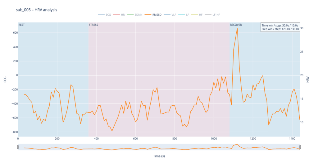
RMSSD
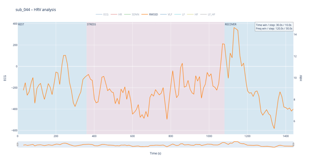
RMSSD is conceptually close to SDNN, but it is calculated as the square root of the mean of the squared differences between successive RR intervals. In essence, RMSSD captures beat-to-beat (“breath-by-breath”) variability, whereas SDNN reflects overall dispersion of intervals within the chosen window. Because of this local focus, we processed RMSSD in a shorter analysis window—30 seconds with a 10-second step—to obtain a curve that is smooth yet sensitive to rapid changes.
The comparative analysis reveals patterns similar to SDNN, with several noteworthy differences. First, in the clinical subjects, the RMSSD range is almost twice as narrow, indicating reduced high-frequency variability—the heart is working in a more “rigid” mode. Second, in both pathological cases, RMSSD rises noticeably toward the end of the protocol: once exercise stops, sharp spikes appear that are virtually absent in the healthy subject. This delayed surge suggests a late engagement of parasympathetic control—the body remains under sympathetic drive for a prolonged period and only during recovery tries to compensate, generating erratic, uneven intervals.
To highlight the heart’s “rigidity,” I plan to map RMSSD to the pitch shift of drums.
Spectral HRV analysis
For spectral HRV analysis the gold-standard window is about five minutes, but in this project we need a compromise between scientific reliability and near-real-time responsiveness. We therefore use a 120-second window with a 60-second step.
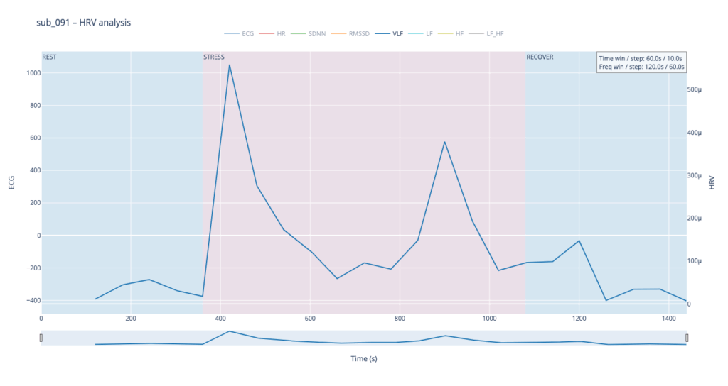
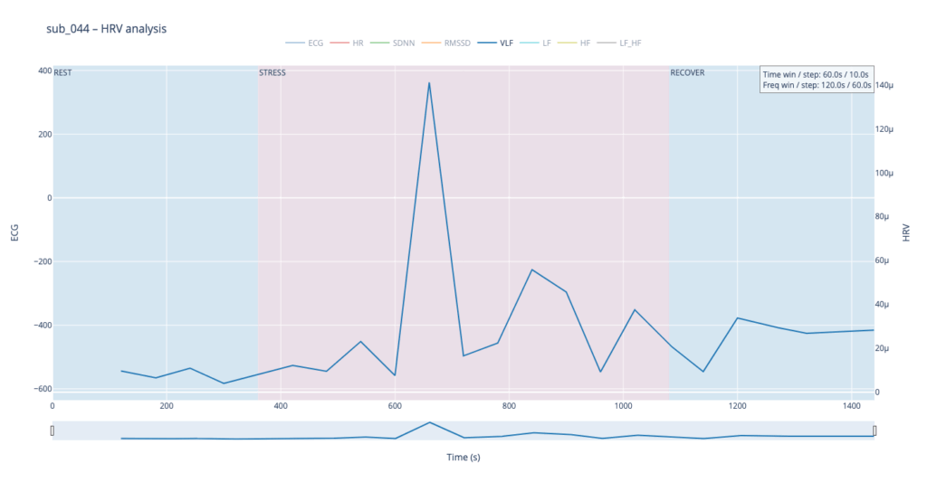
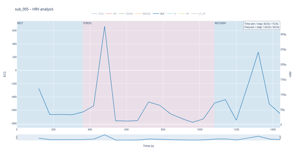
VLF
Within such a short segment, the VLF band (0.003–0.04 Hz)—which is thought to reflect very slow regulatory processes such as hormonal release and thermoregulation—cannot be interpreted with the same statistical confidence as in traditional five-minute blocks. Even so, the plots still reveal that surges in VLF power tend to appear just before rises in heart-rate amplitude. In our context that timing may hint at micro-shifts in core temperature or other slow-acting homeostatic mechanisms that prime the cardiovascular system for the upcoming workload.
VLF → Sub-bass “body boil” layer We will map the slow-acting VLF band to a very low sub-bass drone in the first octave (≈ 30-60 Hz). As VLF power rises the pitch of this bass note is gently shifted upward by a few semitones and a subtle vibrato (slow LFO) is added. The result feels like liquid starting to simmer: higher VLF = hotter “water,” faster wobble, and a slightly higher fundamental. A pre-recorded low-frequency sample (e.g., pitched-down kettle rumble) can sit under the main mix; its playback pitch follows the same VLF curve to reinforce the sensation. When VLF falls, both pitch and vibrato relax, letting the bass settle back to its calm, foundational tone. This approach sonically frames VLF as the deep thermal undercurrent of the body.
LF & HF
Low-Frequency (LF, 0.04–0.15 Hz) and High-Frequency (HF, 0.15–0.40 Hz) power curves mirror the behavior we already saw with SDNN and RMSSD. That is perfectly logical: SDNN and LF both track activity of the sympathetic branch, which dominates under stress—heart rate accelerates, blood pressure rises, LF climbs. Conversely, HF and RMSSD follow the parasympathetic (“vagal”) branch: as the body relaxes, the heart slows, breathing deepens, and HF increases.
Patient 091 delivers a textbook illustration of that theory. At rest his HF overtops LF, but the moment exercise begins the autonomic balance flips—LF jumps above HF and keeps climbing, whereas HF rises more modestly and then drops back near the end, underscoring how hard it is for his system to settle.
By contrast, our other symptomatic patients (044 and 005) show LF dominating HF throughout, signalling a chronically tense autonomic state.
The healthy subject 115 starts with LF and HF almost equal; as effort mounts the gap widens in a smooth, orderly fashion.
Sonically, LF and HF make a natural complement to the VLF layer. We can map their absolute values to pitch in the second octave while using the LF/HF ratio to shape timbre—blending from a pure sine wave toward an edgier saw-like texture. When LF/HF is below 2, the sound stays near sine (calm, vagal tone); as the ratio exceeds 2, it becomes increasingly “saw-toothed,” evoking sympathetic arousal. Also, with this parameter, I would like to control the music scale from major to minor.
In practice, we see 115 and 091 resting in the neutral range and pushing upward only during exercise—the difference being that 115 ascends gradually, whereas 091 leaps. Both glide back to baseline once the task ends.
Patients 044 and 005, however, begin with ratios already high and jittering, telegraphing their persistent sympathetic load.
The next stage will be to develop an algorithm that converts these metrics into MIDI messages that can be mapped to parameters inside a DAW, or, alternatively, to build a SuperCollider or Pure Data patch implementing the same control scheme.
Before we can compare a “healthy” and a “clinical” heart, we first need a small tool-chain that does three things automatically:
detects each normal-to-normal (NN) beat in a raw ECG trace,
converts those beats into the core HRV metrics (HR, SDNN, RMSSD, VLF, LF, HF, LF/HF) and
plots every curve on an interactive dashboard so that trends can be inspected side-by-side.
Because the long-term goal is a live installation (eventually driving MIDI or other real-time mappings), the script is written from the start in a sliding-window style: at every step it re-computes each metric over a moving chunk of data. Fast-changing variables such as heart-rate itself can use short windows and small hops; spectral indices need at least a five-minute span to remain physiologically trustworthy. Shortening that span may make the curves look “lively,” but it also distorts the underlying autonomic picture and breaks any attempt to compare one participant with another. The code therefore lets the user set an independent window length and step size for the time-domain group and for the frequency-domain group. Let’s take a closer look at the code. If you want to see the full, visit: https://github.com/ninaeba/EmbodiedResonance
1. Imports and global parameters
import argparse
import sys
from pathlib import Path

import numpy as np
import pandas as pd
import plotly.graph_objs as go
import scipy.signal as sg
import neurokit2 as nk
argparse – give the script a tiny command-line interface so we can point it at any raw ECG CSV.
NumPy / pandas – basic numeric work and table handling.
Butterworth 0.5–40 Hz is a widely used cardiology band-pass that suppresses baseline wander and high-frequency EMG, yet leaves the QRS complex untouched.
60s time-domain window strikes a balance: long enough to tame noise, short enough for semi-real-time trend tracking.
300s spectral window is deliberately longer; the literature shows that the lower bands (especially VLF) are unreliable below ~5 min.
FGRID – dense frequency grid (1 mHz spacing) for a smoother Lomb curve.
3. ECG helper class – load, (optionally) filter, detect R-peaks
load – reads the CSV into a flat float vector and sanity-checks that we have >10 s of data.
filt – if the --nofilt flag is absent, applies a 4-th-order zero-phase Butterworth band-pass (via filtfilt) so that the baseline drift of slow breathing (or cable motion) does not trick the peak detector.
r_peaks – delegates the hard work to neurokit2.ecg_process, which combines Pan-Tompkins-style amplitude heuristics with adaptive thresholds; returns index positions and their timing in seconds.
time_metrics converts every RR sub-series into three classic metrics – HR (beats/min), SDNN (overall beat-to-beat spread, ms), RMSSD (short-term jitter, ms).
Why Lomb–Scargle instead of Welch? The RR intervals are unevenly spaced by definition.
Welch needs evenly sampled tachograms or heavy interpolation → can distort the spectrum.
Lomb operates directly on irregular timestamps, preserving low-frequency content even if breathing or motion momentarily speeds up/slows down the heart.
lomb_bandpowers:
Runs scipy.signal.lombscargle on de-trended RR values.
Integrates power inside canonical VLF / LF / HF bands.
Computes LF/HF ratio, but guards against division by tiny HF values.
time_series / freq_series slide a window (120 s or 300 s) across the experiment, jump every 30 s, calculate metrics, and store the mid-window timestamp for plotting.
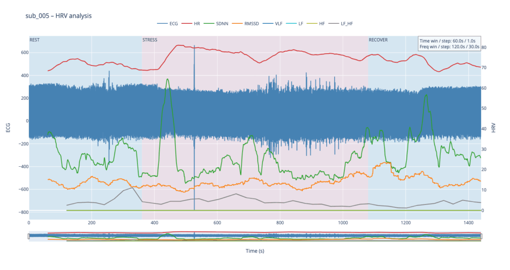
compute finally stitches time-domain and frequency-domain rows onto a 1-second master grid so that all curves overlay cleanly.
Left y-axis = filtered ECG trace for QC (do peaks line up?).
Right y-axis = every HRV curve.
Built-in range-slider lets you scrub the 24-minute protocol quickly.
Hover shows exact numeric values (handy when you are screening anomalies).
different backgrounds for phases
7. CLI wrapper
if __name__ == '__main__':
    main()
Inside main() we parse the file name and the --nofilt flag, run the whole pipeline, save the HRV table as a CSV sibling (same stem, suffix .hrv_lomb.csv) and open the Plotly window.
The four summary plots included below are therefore not an end-point but a launch-pad: they give us a quick visual fingerprint of each participant’s autonomic response, and will serve as the reference material for deeper statistical comparison, pattern-searching, and—ultimately—the data-to-sound (or other real-time) mappings we plan to build next.
Heart-rate variability, or HRV, is the tiny, natural wobble in the time gap from one heartbeat to the next. It exists because two automatic “pedals” are always tugging at the heart. One pedal is the sympathetic system, the same chemistry that makes your pulse race when you are startled. The other pedal is the vagus-driven parasympathetic system, the brake that slows the heart each time you breathe out or settle into a chair. The more freely these pedals can trade places, the more variable those beat-to-beat spacings become. HRV is therefore a quick, non-invasive way to listen to how relaxed, alert, or exhausted the body is.
When we measure HRV we usually pull out a few headline numbers.
SDNN is the overall statistical spread of beat intervals during a slice of time, for example one minute. A wide spread means the heart is flexible and ready to react. A very narrow spread means the system is locked in one gear, as happens in chronic stress or heart failure.
RMSSD zooms in on the jump from one beat to the very next, averages those jumps, and reflects how strongly the vagus brake is speaking. During slow, deep breathing RMSSD grows larger; during mental tension or sleep deprivation it falls.
Frequency-domain measures treat the heartbeat trace like a piece of music and ask how loud each note is. Very-low-frequency power, or VLF, comes from extremely slow body rhythms such as hormone cycles and temperature regulation. Low-frequency power, or LF, sits in the middle and rises when the sympathetic pedal is pressed, for example in the first minute of exercise or during mental arithmetic. High-frequency power, or HF, sits exactly at breathing speed and is almost pure vagus activity: it swells during calm, diaphragmatic breathing and shrinks when breathing is shallow or hurried. A simple way to summarise the tug-of-war is the LF-to-HF ratio. When the sympathetic pedal dominates the ratio climbs; when the vagus brake dominates the ratio slides downward.
In a healthy, rested adult who is quietly seated the heart rate is steady but not rigid. SDNN and RMSSD show a modest but clear jitter, HF power pulses in step with the breath, LF is similar in size to HF, and the LF/HF ratio hovers around one or two. If the same person begins brisk walking heart rate rises, HF power fades, LF power grows, and the LF/HF ratio can shoot above five. During slow breathing meditation RMSSD and HF surge while LF/HF drops below one. In someone with chronic anxiety or PTSD the resting pattern is different: SDNN and RMSSD are low, HF is thin, LF/HF is already high before any task, and it climbs even higher during mild stress. The pattern can be even flatter in advanced heart disease, where both pedals are weak and total HRV is minimal.
Put simply, HRV lets us watch the nervous system’s soundtrack: fast notes reflect breathing and relaxation, mid-notes reflect alertness, and the overall volume tells us how much capacity the system still has in reserve.
The raw material for every HRV metric is the NN-interval sequence: NNi is the time in seconds between two consecutive normal (sinus) beats.
SDNN is the standard deviation of that sequence.
SDNN = √[ Σ (NNi – NN̄)² / (N – 1) ] Units are milliseconds because the intervals are expressed in ms. A resting, healthy adult who sits quietly will usually show an SDNN between roughly 30 ms and 50 ms. Endurance athletes can sit in the 60–90 ms range, while chronically stressed or cardiac patients may drift below 20 ms.
RMSSD focuses on the beat-to-beat jump and is dominated by parasympathetic (vagal) tone.
RMSSD = √[ Σ ( NNi – NNi-1 )² / (N – 1) ] Again the unit is milliseconds. Typical resting values in a calm, healthy adult are about 25–40 ms. Slow breathing, a nap, or meditation can push it up toward 60 ms, whereas sustained mental effort, anxiety, sleep deprivation, or PTSD often pull it down below 15 ms.
Frequency-domain indices start from the same NN series but first convert it into a power-spectrum, most accurately with a Lomb–Scargle periodogram when the points are unevenly spaced:
P(f) = (1/2σ²) { [ Σ NNi cos ωi ]² / Σ cos² ωi + [ Σ NNi sin ωi ]² / Σ sin² ωi } where ω = 2πf and f is scanned from 0.003 Hz upward.
Power is then integrated over preset bands and reported in ms² because it represents variance of the interval series per hertz.
Very-low-frequency power VLF integrates P(f) from 0.003 Hz to 0.04 Hz. In a healthy resting adult VLF is often 500–1500 ms². Because the mechanisms behind VLF (thermoregulation, hormones, renin-angiotensin cycle) change only slowly, values can drift greatly between individuals and between days.
Low-frequency power LF integrates P(f) from 0.04 Hz to 0.15 Hz. A quiet, healthy adult usually sits near 300–1200 ms². LF rises when the sympathetic accelerator is pressed, for example during the first few minutes of exercise or a stressful mental task.
High-frequency power HF integrates P(f) from 0.15 Hz to 0.40 Hz, exactly the normal breathing range. Calm diaphragmatic breathing drives HF toward 400–1200 ms², whereas rapid or shallow breathing in anxiety or hard exercise cuts HF sharply, sometimes below 100 ms².
LF/HF is the simple ratio LF ÷ HF. At rest a ratio near 1–2 suggests a balanced tug-of-war. If the ratio soars above 5 the sympathetic branch is clearly on top; if it falls below 0.5 the vagus brake is dominating (seen in deep meditation or in some fainting-prone individuals).
All of these numbers rise and fall in real time as the two branches of the autonomic nervous system jostle for control, so plotting them across the exercise-rest protocol lets us see how quickly and how strongly each person’s physiology reacts and recovers.
Metric
Units
What It Reflects (plain-language)
Typical Resting Range in Healthy Adults*
When It Runs High (what that often means)
When It Runs Low (what that can signal)
Mean Heart Rate (HR)
beats per minute (bpm)
How fast the heart is beating on average
50 – 80 bpm
Physical effort, fever, anxiety, dehydration
Excellent cardiovascular fitness, medications that slow the heart
SDNN
milliseconds (ms)
Overall “spread” of beat-to-beat intervals—long-term autonomic flexibility
40 – 60 ms
Good recovery, calm alertness, athletic conditioning
Chronic stress, heart disease, PTSD, over-fatigue
RMSSD
ms
Very short-term vagal (rest-and-digest) shifts from one beat to the next
25 – 45 ms
Deep relaxed breathing, meditation, lying down
Sympathetic overdrive, poor sleep, depression
VLF Power
ms²
Very-slow oscillations (< 0.04 Hz) tied to long hormonal / thermoregulatory rhythms
600 – 2000 ms²
Possible inflammation, overtraining, sustained stress load
At the current stage of the project, before engaging with real-time biofeedback sensors or integrating hardware systems, I deliberately chose to begin with a simulation-based exploration using publicly available physiological datasets. This decision was grounded in both practical and conceptual motivations. On one hand, working with curated datasets provides a stable, low-risk environment to test hypotheses, establish workflows, and identify relevant signal characteristics. On the other hand, it also offered an opportunity to engage critically with the structure, semantics, and limitations of real-world psychophysiological recordings—particularly in the context of trauma-related conditions.
My personal interest in trauma physiology, shaped by lived experience during the war in Ukraine, has influenced the conceptual direction of this work. I was particularly drawn to understanding how conditions such as post-traumatic stress disorder (PTSD) might leave measurable traces in the body—traces that could be explored not only scientifically, but also sonically and artistically. This interest was further informed by reading The Body Keeps the Score by Bessel van der Kolk, which inspired me to look for empirical signals that reflect internal states which often remain inaccessible through language alone.
With this perspective in mind, I selected a large dataset focused on stress-induced myocardial ischemia as a starting point. Although the dataset was not originally designed to study PTSD, it includes a diverse group of participants—among them individuals diagnosed with PTSD, as well as others with complex comorbidities such as coronary artery disease and anxiety-related disorders. The richness of this cohort, combined with the inclusion of multiple biosignals (ECG, respiration, blood pressure), makes it a promising foundation for exploratory analyses.
Rather than seeking definitive conclusions at this point, my aim is to uncover what is possible—to understand which physiological patterns may hold relevance for trauma detection, and how they might be interpreted or transformed into expressive modalities such as sound or movement. This stage of the project is therefore best described as investigative and generative: it is about opening up space for experimentation and reflection, rather than narrowing toward specific outcomes.
Data Preparation and Extraction of Clinical Metadata from JSON Records
To efficiently identify suitable subjects for simulation, I first downloaded a complete index of data file links provided by the repository. Using a regular expression-based filtering mechanism implemented in Python, I programmatically extracted only those links pointing to disease-related JSON records for individual subjects (i.e., files following the pattern sub_XXX_disease.json). This was performed using a custom script (see downloaded_disease_files.py) which reads the full list of URLs from a text file and downloads the filtered subset into a local directory. A total of 119 such JSON records were retrieved.
Following acquisition, a second Python script (summary.py) was used to parse each JSON file and consolidate its contents into a single structured table. Each JSON file contained binary and categorical information corresponding to specific diagnostic criteria, including presence of PTSD, angina, stress-induced ischemia, pharmacological responses, and psychological traits (e.g., anxiety and depression scale scores, Type D personality indicators).
The script extracted all available key-value pairs and added a subject_id field derived from the filename. These entries were stored in a pandas DataFrame and exported to a CSV file (patients_disease_table.csv). The resulting table forms the basis for all subsequent filtering and selection of patient profiles for simulation.
This pipeline enabled me to rapidly triage a heterogeneous dataset by transforming a decentralized JSON structure into a unified tabular format suitable for further querying, visualization, and real-time signal emulation.
Group Selection and Dataset Subsetting
In order to meaningfully simulate and compare physiological responses, I manually selected a subset of subjects from the larger dataset and organized them into four distinct groups based on diagnostic profiles derived from the structured disease table:
Healthy group: Subjects with no recorded psychological or cardiovascular abnormalities.
Mental health group: Subjects presenting only with psychological traits such as elevated anxiety, depressive symptoms, or Type D personality, but without ischemic or cardiac diagnoses.
PTSD group: Subjects with a verified PTSD diagnosis, often accompanied by anxiety traits and non-obstructive angina, but without broader comorbidities.
Clinically sick group: Subjects with extensive multi-morbidity, showing positive indicators across most of the diagnostic criteria including ischemia, psychological disorders, and cardiovascular dysfunctions.
This manual classification enabled targeted downloading of signal data for only those subjects who are of particular interest to the ongoing research.
A custom Python script was then used to selectively retrieve only the relevant signal files—namely, 500 Hz ECG recordings from three phases (rest, stress, recovery) and the corresponding clinical complaint JSON files. The script filters a list of raw download links by matching both the subject ID and filename patterns. Each file is downloaded into a separate folder named after its respective group, thereby preserving the classification structure for downstream analysis and simulation.
Preprocessing of Raw ECG Signal Files
Upon downloading the raw signal files for the selected subjects, several structural and formatting issues became immediately apparent. These challenges rendered the original data format unsuitable for direct use in real-time simulation or further analysis. Specifically:
Scientific Notation Format All signal values were encoded in scientific notation (e.g., 3.2641e+02), requiring transformation into standard integer format suitable for time-domain processing and sonification.
Flattened and Fragmented Data Each file contained a single long sequence of values with no clear delimiters or column headers. In some cases, the formatting introduced line breaks within numbers, further complicating parsing and extraction.
Twelve-Lead ECG in a Single File The signal for all 12 ECG leads was stored in a single continuous stream, without metadata or segmentation markers. The only known constraint was that the total length of the signal was always divisible by 12, implying equal-length segments per lead.
Separated Recording Phases Data for each subject was distributed across three files, each corresponding to one of the experimental phases: rest, stress, and recovery. For the purposes of this project—particularly real-time emulation and comparative analysis—I required a single, merged file per lead containing the full time course across all three conditions.
Solution: Custom Parsing and Lead Separation Script
To address these challenges, I developed a two-stage Python script to convert the raw .csv files into a structured and usable format:
Step 1: Parsing and Lead Extraction The script recursively traverses the directory tree to identify ECG files by filename patterns. For each file:
The ECG phase (rest, stress, or recover) is inferred from the filename.
The subject ID is extracted using regular expressions.
All scientific-notation numbers are matched and converted into integers. Unrealistically large values (above 10,000) are filtered out to prevent corruption.
The signal is split into 12 equally sized segments, corresponding to the 12 ECG leads. Each lead is saved as a separate .csv file inside a folder structure organized by subject and phase.
Step 2: Lead-Wise Concatenation Across Phases Once individual leads for each phase were saved, the script proceeds to merge the rest, stress, and recovery segments for each lead:
For every subject, it locates the three corresponding files for each lead.
These files are concatenated vertically (along the time axis) to form a continuous signal.
The resulting merged signals are saved in a dedicated combined folder per subject, with filenames that indicate the lead number and sampling rate.
This conversion pipeline transforms non-tabular raw data into standardized time series inputs suitable for further processing, visualization, or real-time simulation.
Manual Signal Inspection and Selection of Representative Subjects
While the data transformation pipeline produced technically readable ECG signals, closer inspection revealed a range of physiological artifacts likely introduced during the original data acquisition process. These irregularities included signal clipping, baseline drift, and abrupt discontinuities. In many cases, such artifacts can be attributed not to software or conversion errors, but to common physiological and mechanical factors—such as subject movement, poor electrode contact, skin conductivity variation due to perspiration, or unstable placement of leads during the recording.
These artifacts are highly relevant from a performative and conceptual standpoint. Movement-induced noise and instability in bodily measurements reflect the lived, embodied realities of trauma, and they may eventually be used as expressive material within the performance itself. However, for the purpose of initial analysis and especially heart rate variability (HRV) extraction, such disruptions compromise signal clarity and algorithmic robustness.
To navigate this complexity, I conducted a manual review of the ECG signals for all 16 selected subjects. Each of the 12 leads per subject was visually examined across the three experimental phases (rest, stress, and recovery). From this process, I identified one subject from each group (healthy, mental health, PTSD, and clinically sick) whose signals displayed the least amount of distortion and were most suitable for initial HRV-focused simulation.
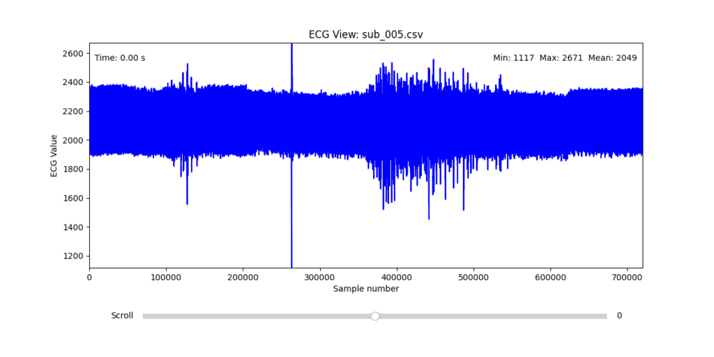
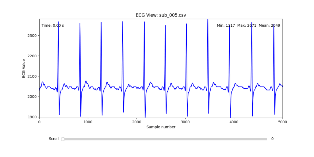
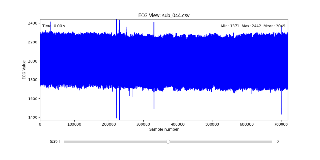
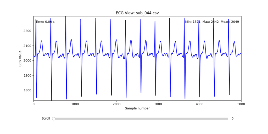
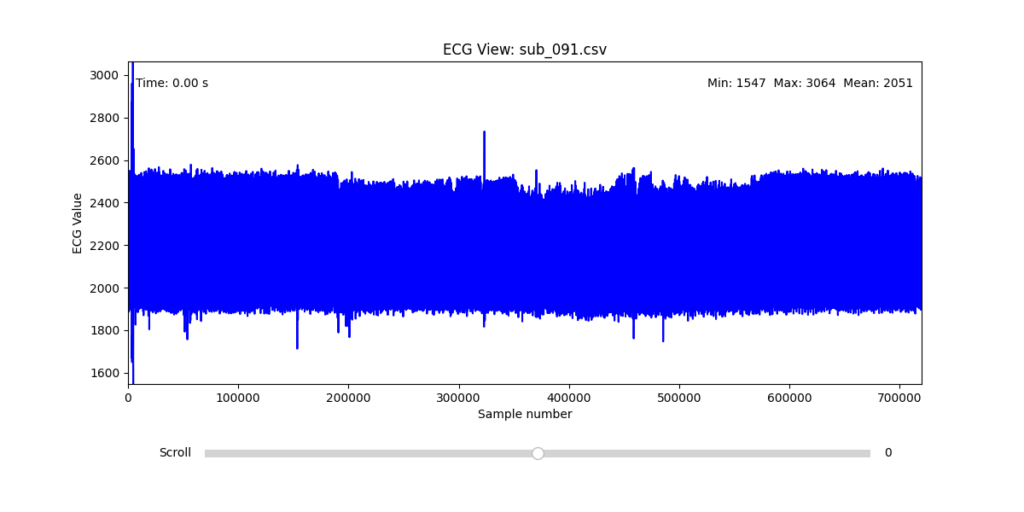
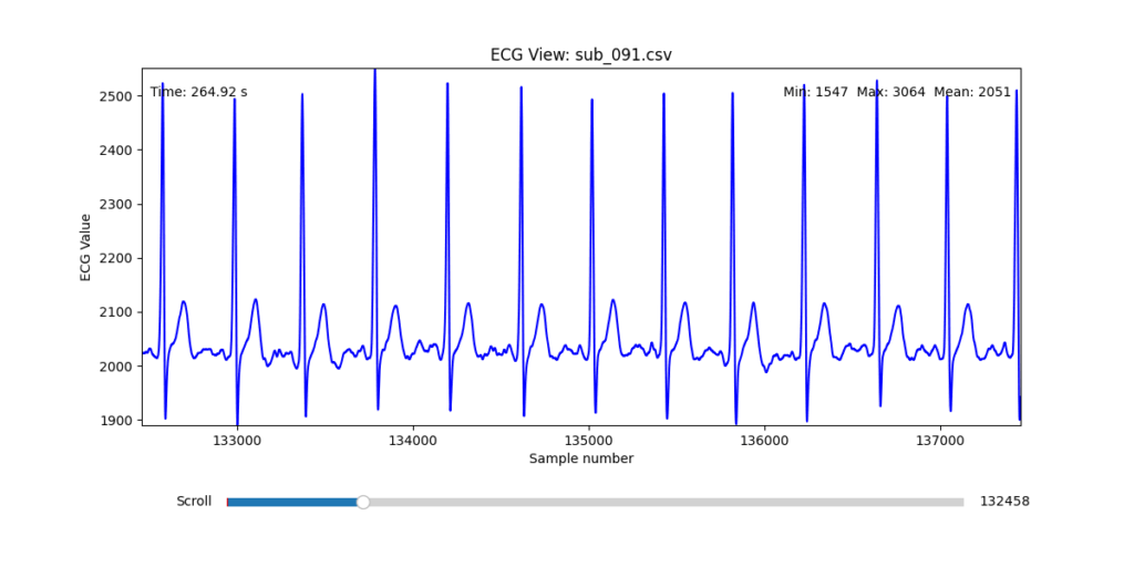
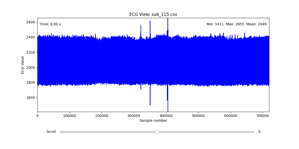
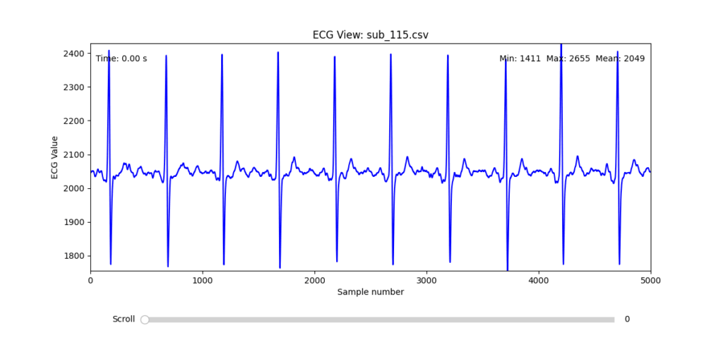
Diagnostic Visualization Tool
To facilitate and streamline this selection process, I implemented a simple interactive visualization tool in Python. This utility allows for scrollable navigation through long ECG recordings, with a resizable window and basic summary statistics (min, max, mean values). It was essential for rapidly identifying where signal corruption occurred and assessing lead quality in a non-automated but highly effective way.
This tool enabled both quantitative assessment and intuitive engagement with the data, providing a necessary bridge between raw measurement and informed experimental design.
Selection of Final Subjects and Optimal ECG Leads
Following visual inspection of all 12 ECG leads across the 16 initially shortlisted subjects, I selected one representative from each diagnostic group whose recordings exhibited the highest signal quality and least interference. The selection was based on manual analysis using the custom-built scrollable ECG viewer, with particular attention given to the clarity and prominence of QRS complexes—a critical factor for accurate heart rate variability (HRV) analysis. The final subjects are: 005, 044, 091, 115:
These signals will serve as the primary input for all upcoming simulation and sonification stages. While artifacts remain an inherent part of physiological measurement—especially in ambulatory or emotionally charged conditions—this selection aims to provide a clean analytical baseline from which to explore more experimental, expressive interpretations in later phases.
References:
Van der Kolk, Bessel A. 2014. The Body Keeps the Score: Brain, Mind, and Body in the Healing of Trauma. New York: Viking.