Experiment IV: Embodied Resonance – plot HRV metrics with python

Before we can compare a “healthy” and a “clinical” heart, we first need a small tool-chain that does three things automatically:

1. detects each normal-to-normal (NN) beat in a raw ECG trace,
2. converts those beats into the core HRV metrics (HR, SDNN, RMSSD, VLF, LF, HF, LF/HF) and
3. plots every curve on an interactive dashboard so that trends can be inspected side-by-side.

Because the long-term goal is a live installation (eventually driving MIDI or other real-time mappings), the script is written from the start in a sliding-window style: at every step it re-computes each metric over a moving chunk of data.
Fast-changing variables such as heart-rate itself can use short windows and small hops; spectral indices need at least a five-minute span to remain physiologically trustworthy. Shortening that span may make the curves look “lively,” but it also distorts the underlying autonomic picture and breaks any attempt to compare one participant with another. The code therefore lets the user set an independent window length and step size for the time-domain group and for the frequency-domain group.
Let’s take a closer look at the code. If you want to see the full, visit: https://github.com/ninaeba/EmbodiedResonance

1. Imports and global parameters

import argparse
import sys
from pathlib import Path

import numpy as np
import pandas as pd
import plotly.graph_objs as go
import scipy.signal as sg
import neurokit2 as nk

• argparse – give the script a tiny command-line interface so we can point it at any raw ECG CSV.
• NumPy / pandas – basic numeric work and table handling.
• scipy.signal – classic DSP tools (Butterworth filter, Lomb–Scargle).
• neurokit2 – robust, well-tested R-peak detector.
• plotly – interactive plotting inside a browser/Notebook; easy zooming for visual QA.

2. Tunable experiment-wide constants

FS_ECG   = 500              # ECG sample-rate (Hz)
BP_ECG   = (0.5, 40)        # band-pass corner frequencies

TIME_WIN, TIME_STEP = 60.0, 1.0   # sliding window for HR / SDNN / RMSSD
FREQ_WIN, FREQ_STEP = 300.0, 30.0   # sliding window for VLF / LF / HF
FGRID = np.arange(0.003, 0.401, 0.001)

BANDS = dict(VLF=(.003, .04), LF=(.04, .15), HF=(.15, .40))

• Butterworth 0.5–40 Hz is a widely used cardiology band-pass that suppresses baseline wander and high-frequency EMG, yet leaves the QRS complex untouched.
• 60s time-domain window strikes a balance: long enough to tame noise, short enough for semi-real-time trend tracking.
• 300s spectral window is deliberately longer; the literature shows that the lower bands (especially VLF) are unreliable below ~5 min.
• FGRID – dense frequency grid (1 mHz spacing) for a smoother Lomb curve.

3. ECG helper class – load, (optionally) filter, detect R-peaks

class ECG:
    def __init__(self, fs=FS_ECG, bp=BP_ECG, use_filter=True):
        ...
    def load(self, fname: Path) -> np.ndarray:
        ...
    def filt(self, sig):
        ...
    def r_peaks(self, sig_f):
        ...

1. load – reads the CSV into a flat float vector and sanity-checks that we have >10 s of data.
2. filt – if the --nofilt flag is absent, applies a 4-th-order zero-phase Butterworth band-pass (via filtfilt) so that the baseline drift of slow breathing (or cable motion) does not trick the peak detector.
3. r_peaks – delegates the hard work to neurokit2.ecg_process, which combines Pan-Tompkins-style amplitude heuristics with adaptive thresholds; returns index positions and their timing in seconds.

4. HRV class – sliding-window metric engine

class HRV:
    ...
    def time_metrics(rr):
        ...
    def lomb_bandpowers(self, rr, t_rr):
        ...
    def time_series(self, r_t):
        ...
    def freq_series(self, r_t):
        ...
    def compute(self, r_t):
        ...

• time_metrics converts every RR sub-series into three classic metrics
  – HR (beats/min), SDNN (overall beat-to-beat spread, ms), RMSSD (short-term jitter, ms).
• Why Lomb–Scargle instead of Welch?
  The RR intervals are unevenly spaced by definition.
  • Welch needs evenly sampled tachograms or heavy interpolation → can distort the spectrum.
  • Lomb operates directly on irregular timestamps, preserving low-frequency content even if breathing or motion momentarily speeds up/slows down the heart.
• lomb_bandpowers:
  1. Runs scipy.signal.lombscargle on de-trended RR values.
  2. Integrates power inside canonical VLF / LF / HF bands.
  3. Computes LF/HF ratio, but guards against division by tiny HF values.
• time_series / freq_series slide a window (120 s or 300 s) across the experiment, jump every 30 s, calculate metrics, and store the mid-window timestamp for plotting.
• compute finally stitches time-domain and frequency-domain rows onto a 1-second master grid so that all curves overlay cleanly.

5. Tiny colour dictionary

COLORS = dict(HR='#d62728', SDNN='#2ca02c', RMSSD='#ff7f0e',
              VLF='#1f77b4', LF='#17becf', HF='#bcbd22', LF_HF='#7f7f7f')

Just cosmetic – keeps HR red, SDNN green, etc., across all subjects so eyeballing becomes effortless.

6. plot() – interactive dashboard

def plot(ecg_f, hrv_df, fs=FS_ECG, title="HRV (Lomb)"):
    ...

• Left y-axis = filtered ECG trace for QC (do peaks line up?).
• Right y-axis = every HRV curve.
• Built-in range-slider lets you scrub the 24-minute protocol quickly.
• Hover shows exact numeric values (handy when you are screening anomalies).

7. CLI wrapper

if __name__ == '__main__':
    main()

Inside main() we parse the file name and the --nofilt flag, run the whole pipeline, save the HRV table as a CSV sibling (same stem, suffix .hrv_lomb.csv) and open the Plotly window.

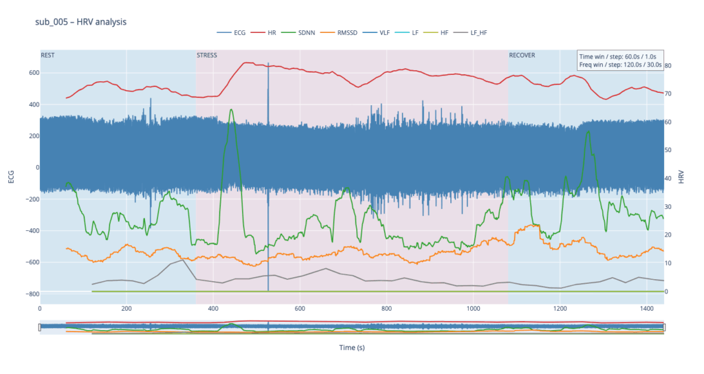
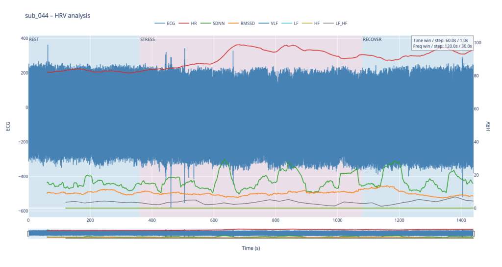
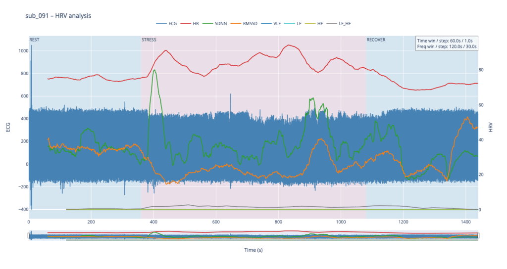
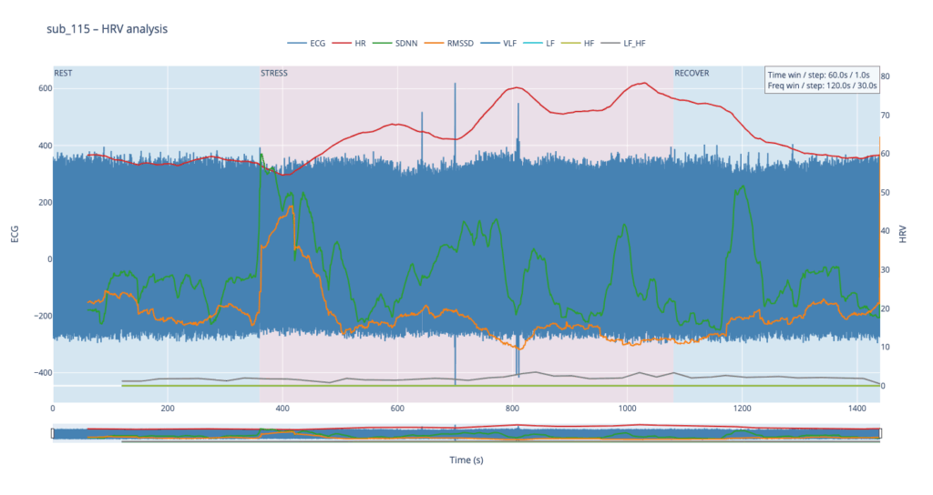
The four summary plots included below are therefore not an end-point but a launch-pad: they give us a quick visual fingerprint of each participant’s autonomic response, and will serve as the reference material for deeper statistical comparison, pattern-searching, and—ultimately—the data-to-sound (or other real-time) mappings we plan to build next.